Comparative and Longitudinal Connectomics

In this vignette, we show how to compare connectomics across multiple single-cell datasets, indepedent of node parcellation. The functions below are able to compare cell-cell signaling topologies across conditions, timepoints, and even across tissues/organs. For demonstration, we use the muscle regeneration dataset from DeMicheli et al. 2020.

Load Dependencies

library(Seurat)
library(Connectome)
library(cowplot)
library(knitr)

Load and Format data

GSE143437_DeMicheli_MuSCatlas_metadata <- read.delim("GSE143437_DeMicheli_MuSCatlas_metadata.txt")
GSE143437_DeMicheli_MuSCatlas_rawdata <- read.delim("GSE143437_DeMicheli_MuSCatlas_rawdata.txt")
raw.data <- GSE143437_DeMicheli_MuSCatlas_rawdata
meta.data <- GSE143437_DeMicheli_MuSCatlas_metadata
rm(GSE143437_DeMicheli_MuSCatlas_rawdata)
rm(GSE143437_DeMicheli_MuSCatlas_metadata)
# Reformat rownames
raw.data.2 <- raw.data[,-1]
rownames(raw.data.2) <- raw.data[,1]
meta.data.2 <- meta.data[,-1]
rownames(meta.data.2) <- meta.data[,1]

Data Structure and Processing

This dataset contains 10x data across 4 timepoints during a muscle injury and regeneration model. Here, we convert the raw counts to a Seurat object, split the data by injury timepoint, and then make the corresponding x4 tissue connectomes.

# Create Seurat Object
musc <- CreateSeuratObject(counts = raw.data.2)
musc <- AddMetaData(musc,metadata = meta.data.2)
Idents(musc) <- musc[['cell_annotation']]

# Identify ligands and receptors which have mapped in the dataset:
connectome.genes <- union(Connectome::ncomms8866_mouse$Ligand.ApprovedSymbol,Connectome::ncomms8866_mouse$Receptor.ApprovedSymbol)
genes <- connectome.genes[connectome.genes %in% rownames(musc)]

# Split by timepoint
data <- SplitObject(musc, split.by = 'injury')
for (i in 1:length(data)){
  data[[i]] <- ScaleData(data[[i]])
}

# Normalize, Scale, and create Connectome:
musc.con <- list()
for (i in 1:length(data)){
  data[[i]] <- NormalizeData(data[[i]])
  data[[i]] <- ScaleData(data[[i]],features = genes)
  musc.con[[i]] <- CreateConnectome(data[[i]],species = 'mouse',p.values = F)
}
names(musc.con) <- names(data)

Note that differential connectomics cannot easily be performed here, because the data has been parcellated into different nodes at different time points.

kable(table(Idents(musc),musc@meta.data$injury))

	Day 0	Day 2	Day 5	Day 7
Anti-inflammatory macrophages	0	0	4839	792
B/T/NK cells	50	0	450	147
Endothelial	2678	317	549	1353
FAPs	2425	583	2591	3161
Mature skeletal muscle	566	0	176	159
Monocytes/Macrophages/Platelets	0	2749	3174	0
MuSCs and progenitors	156	0	1641	786
Neural/Glial/Schwann cells	266	0	0	148
Pro-inflammatory macrophages	0	1315	0	0
Resident Macrophages/APCs	164	560	820	304
Smooth muscle cells	509	0	0	387
Tenocytes	214	0	0	409

This is okay! This is exactly the use-case we have designed CompareCentrality for.

Comparing mechanistic centrality across disparate datasets

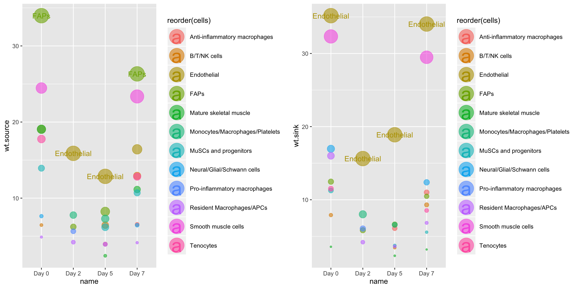
CompareCentrality is similar to Centrality, but instead of grouping in the input network into sub-networks based by a requested group.by term, it analyzes a list of input networks and compares their signaling topologies side-by-side. This allows comprehensive ranking of signal producers and receivers within a chosen network across multiple tissue systems (in this case, x4 timepoints following injury). Here, we analyze the entire VEGF signaling family network across all timepoints:

# Comparative centrality
CompareCentrality(musc.con,
                  weight.attribute = 'weight_norm',
                  modes.include = 'VEGF')

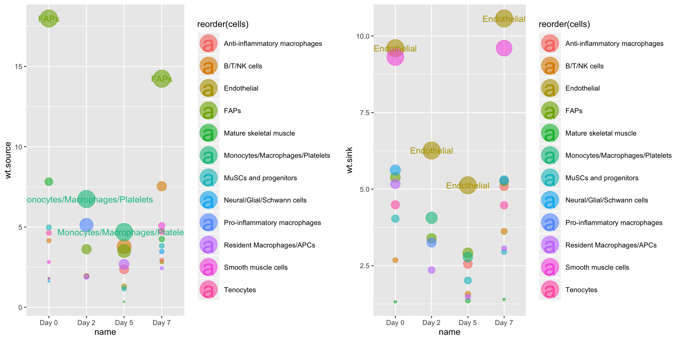
We can also use this function to look at network centrality for only those edges involving a specific gene:

CompareCentrality(musc.con,
                  weight.attribute = 'weight_norm',
                  #min.pct = 0.1,
                  features = 'Vegfa')

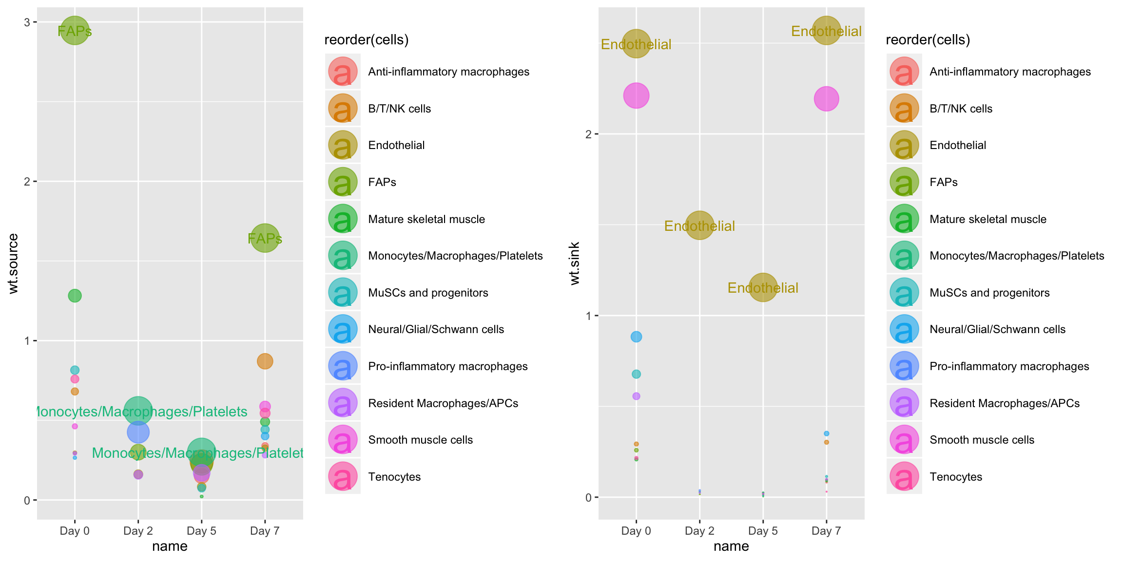
Or, we can use CompareCentrality to quantify signaling centrality across all timepoints for only a specific mechanism:

CompareCentrality(musc.con,
                  weight.attribute = 'weight_norm',
                  #min.pct = 0.1,
                  mechanisms.include = 'Vegfa - Flt1')

Longitudinal Ligand - Receptor Contours

It should be noted that the Connectome data frames lend themselves well to longitudinal ggplotting which allow observation of trends over time. Since we already have a dataset loaded which captures 4 timepoints in a post-injury regeneration model, let’s take a look at how certain ligand - receptor topologies change over time.

Define a longitudinal plotting function

First, let’s define a simple function to format our data

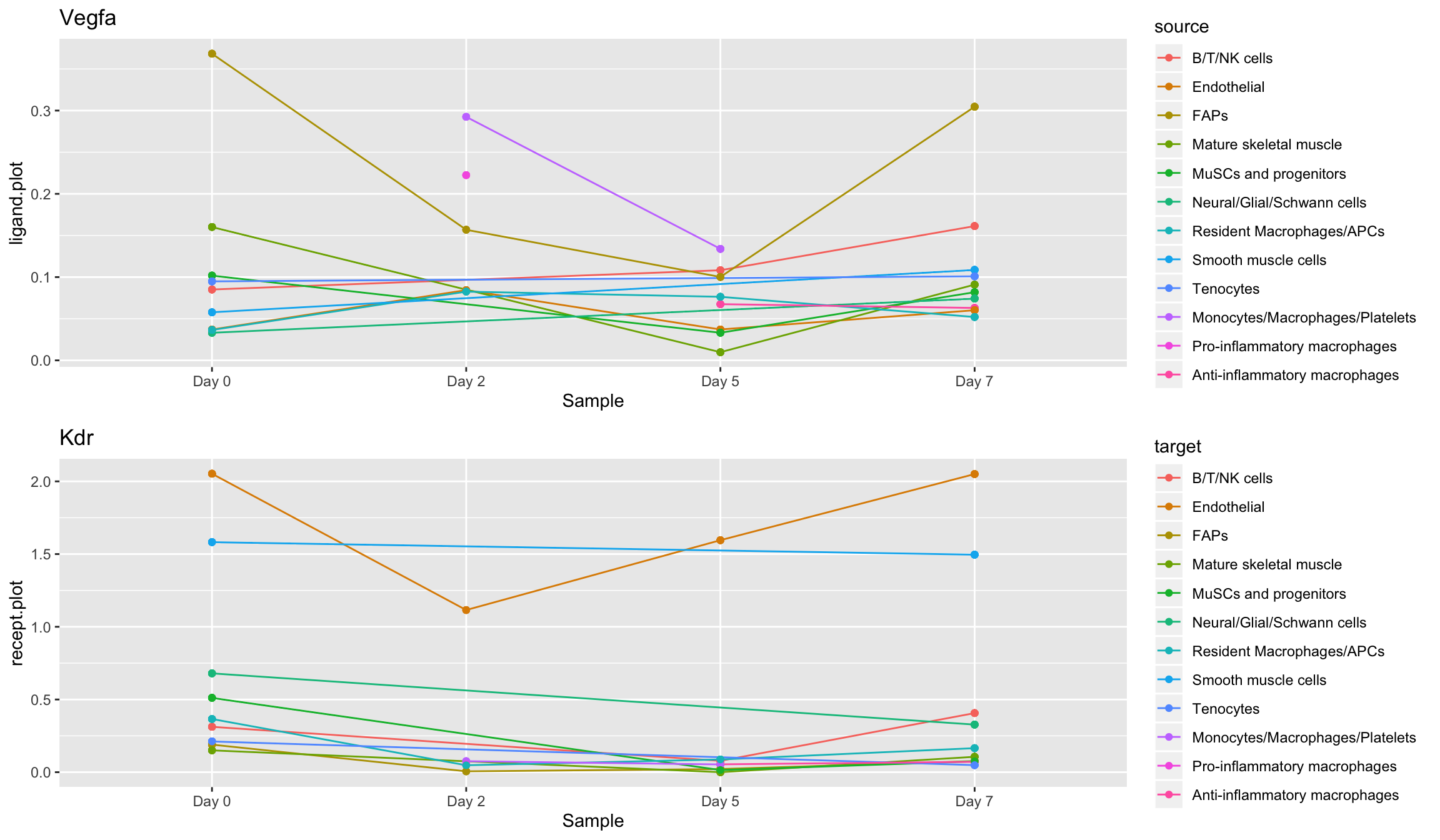
Longitudinal <- function(con.list,LOI,ROI,use.scaled = F,...){
  data <- data.frame()
  for (i in 1:length(con.list)){
    con.list[[i]]$sample.name <- names(con.list)[i]
    data <- rbind(data,con.list[[i]])
  }

  temp <- subset(data,ligand == LOI & receptor == ROI)

  if(use.scaled == F){
    temp$ligand.plot <- temp$ligand.expression
    temp$recept.plot <- temp$recept.expression
  }else{
    temp$ligand.plot <- temp$ligand.scale
    temp$recept.plot <- temp$recept.scale
  }

  p1 <- ggplot(temp,aes(x = factor(sample.name, levels = names(con.list)),
                        y = ligand.plot,group = source,color = source)) +
    geom_line() +
    geom_point() +
    xlab('Sample') +
    ggtitle(LOI)
  p2 <- ggplot(temp,aes(x = factor(sample.name, levels = names(con.list)),
                        y = recept.plot,group = target,color = target)) +
    geom_line() +
    geom_point() +
    xlab('Sample') +
    ggtitle(ROI)

  plot_grid(p1,p2,ncol=1)
}

Longitudinal plots

Now we’re prepared to observe ligand trends and receptor trends over time, for each cell type which was defined in the original single-cell data. We can see from the following plots that FAP cells only display high levels of Vegfa in their homeostatic states (Day 0 and Day 7), while immediately post-injury and during hearing (Day 2 and Day 5) a Monocyte/Macropahge population arises which appears to temporarily support Vegfa secretion:

Longitudinal(musc.con,LOI = 'Vegfa',ROI = 'Kdr')

Micha Sam Brickman Raredon