Connectome can be used to identify and visualize major perturbed cell-cell communication pathways in A:B comparisons of complex tissue systems.

Load dependencies

library(Seurat)
library(SeuratData)
library(Connectome)
library(ggplot2)
library(cowplot)
library(ComplexHeatmap)

Load Data

To demonstrate differential connectomics using Connectome, we will use the interferon-stimulated vs. control PBMC data distributed by SeuratData:

InstallData('ifnb')
data('ifnb')
table(Idents(ifnb))
#> 
#> IMMUNE_CTRL IMMUNE_STIM 
#>        6548        7451
Idents(ifnb) <- ifnb[['seurat_annotations']]
table(Idents(ifnb))
#> 
#>    CD14 Mono  CD4 Naive T CD4 Memory T    CD16 Mono            B 
#>         4362         2504         1762         1044          978 
#>        CD8 T  T activated           NK           DC  B Activated 
#>          814          633          619          472          388 
#>           Mk          pDC        Eryth 
#>          236          132           55

Scale and make connectomes

Connectomic networks must first be calculated for each tissue system separately. To do so:

# First identify ligands and receptors which have mapped in the dataset:
connectome.genes <- union(Connectome::ncomms8866_human$Ligand.ApprovedSymbol,Connectome::ncomms8866_human$Receptor.ApprovedSymbol)
genes <- connectome.genes[connectome.genes %in% rownames(ifnb)]
# Split the object by condition:
ifnb.list <- SplitObject(ifnb,split.by = 'stim')
# Normalize, Scale, and create Connectome:
ifnb.con.list <- list()
for (i in 1:length(ifnb.list)){
  ifnb.list[[i]] <- NormalizeData(ifnb.list[[i]])
  ifnb.list[[i]] <- ScaleData(ifnb.list[[i]],features = rownames(ifnb.list[[i]]))
  ifnb.con.list[[i]] <- CreateConnectome(ifnb.list[[i]],species = 'human',p.values = F)
}
names(ifnb.con.list) <- names(ifnb.list)

Make differential connectome

The two global signaling networks can then be directly compared. Here, we do so using the function DifferentialConnectome. For this functon to run, the two systems must be parcellated in exactly the same way (the same cell types must be present in both) and the rownames (genes) of the original DGE matrices must be identical.

diff <- DifferentialConnectome(ifnb.con.list[[1]],ifnb.con.list[[2]])

Find edges of statistical significance

Because we are dealing with single-cell data, we can leverage the data structure to identify which ligands and receptors, in which cell populations, have changed in a statistically significant fashion. One way to do this:

# Stash idents and make new identities which identify each as stimulated vs. control
celltypes <- as.character(unique(Idents(ifnb)))
celltypes.stim <- paste(celltypes, 'STIM', sep = '_')
celltypes.ctrl <- paste(celltypes, 'CTRL', sep = '_')
ifnb$celltype.condition <- paste(Idents(ifnb), ifnb$stim, sep = "_")
ifnb$celltype <- Idents(ifnb)
Idents(ifnb) <- "celltype.condition"

# Identify which ligands and receptors, for which cell populations, have an adjusted p-value < 0.05 based on a Wilcoxon rank test
diff.p <- data.frame()
for (i in 1:length(celltypes)){
  temp <- FindMarkers(ifnb,
                      ident.1 = celltypes.stim[i],
                      ident.2 = celltypes.ctrl[i],
                      verbose = FALSE,
                      features = genes,
                      min.pct = 0,
                      logfc.threshold = 0)
  temp2 <- subset(temp, p_val_adj < 0.05)
  if (nrow(temp2)>0){
  temp3 <- data.frame(genes = rownames(temp2),cells = celltypes[i])
  diff.p <- rbind(diff.p, temp3)
  }
}
diff.p$cell.gene <- paste(diff.p$cells,diff.p$genes,sep = '.')

# Filter differential connectome to only include significantly perturbed edges
diff$source.ligand <- paste(diff$source,diff$ligand,sep = '.')
diff$target.receptor <- paste(diff$target,diff$receptor,sep = '.')
diff.sub <- subset(diff,source.ligand %in% diff.p$cell.gene & target.receptor %in% diff.p$cell.gene)

Differential Scoring Plot

Differential connectomics are challenging to visualize, because every differential edge takes data from 4 places: the ligand expression in both the control and test condition, and the receptor expression in the control and test condition. Further, a single ligand can hit multiple receptors and vice-versa. One way to visualize this data is with edge-aligned heatmaps. Here, we use the function DifferentialScoringPlot to create three aligned heatmaps: one showing the ligand log fold change, one showing the receptor log fold change, and one showing a ‘perturbation score’ which is the product of the absolute values of the data in the first two plots. This helps to identify those edges which both pass the desired expression thresholds in at least one of the systems, and are highly perturbed in the A:B comparison.

DifferentialScoringPlot(diff.sub,min.score = 1,min.pct = 0.1,infinity.to.max = T)

Differential Circos Plots

Since the above plot is not particularly concise, we have built DifferentialCircos, which draws circos plots for a differential connectome. This plot type makes use of the perturbation score, which is always positive, by design. However, in conenctomic data, there are 4 separate classes of perturbations, as both the ligand and the receptor can either be differentially increased or decreased. Here, we look at the above edgelist (which is shown in full in the DifferentialScoringPlot) and investigate each type of perturbation in turn:

Ligand and receptor are both UP:

diff.up.up <- subset(diff.sub,ligand.norm.lfc > 0 & recept.norm.lfc > 0 )
CircosDiff(diff.up.up,min.score = 2,min.pct = 0.1,lab.cex = 0.4)

Ligand is UP and receptor is DOWN:

diff.up.down <- subset(diff.sub,ligand.norm.lfc > 0 & recept.norm.lfc < 0 )
CircosDiff(diff.up.down,min.score = 2,min.pct = 0.1,lab.cex = 0.4)

Ligand is DOWN and receptor is UP:

diff.down.up <- subset(diff.sub,ligand.norm.lfc < 0 & recept.norm.lfc > 0 )
CircosDiff(diff.down.up,min.score = 2,min.pct = 0.1,lab.cex = 0.4)

Ligand and receptor are both DOWN:

diff.down.down <- subset(diff.sub,ligand.norm.lfc < 0 & recept.norm.lfc < 0 )
CircosDiff(diff.down.down,min.score = 2,min.pct = 0.1,lab.cex = 0.4)

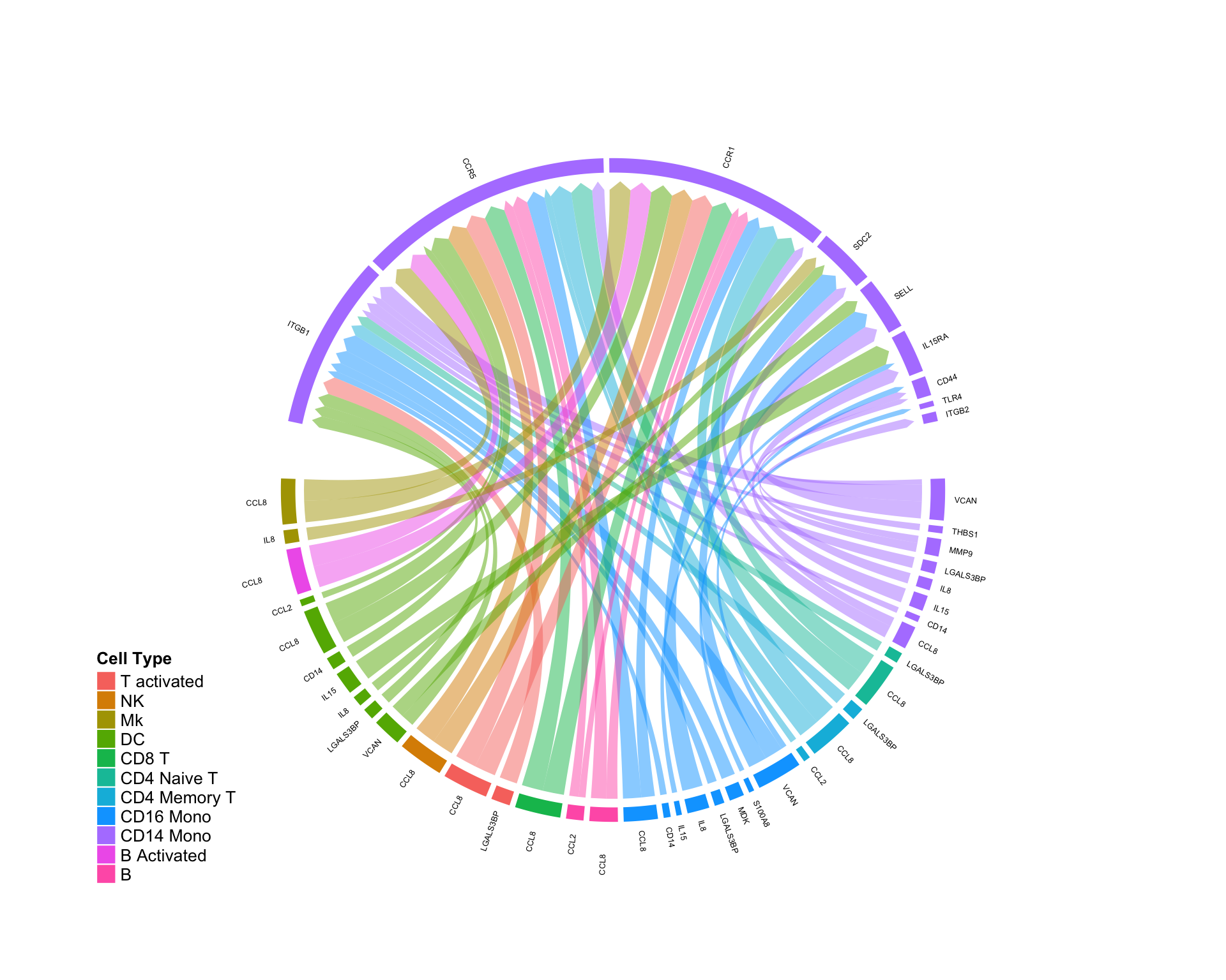
Focusing on specific cell-cell interactions:

We can also use DifferentialCircos to quantify edge perturbation within a specific subset or community of cells:

CircosDiff(diff.sub,min.score = 2,min.pct = 0.1,lab.cex = 0.4,
           sources.include = c('pDC','CD8 T','B'),targets.include = c('CD16 Mono','CD14 Mono'))

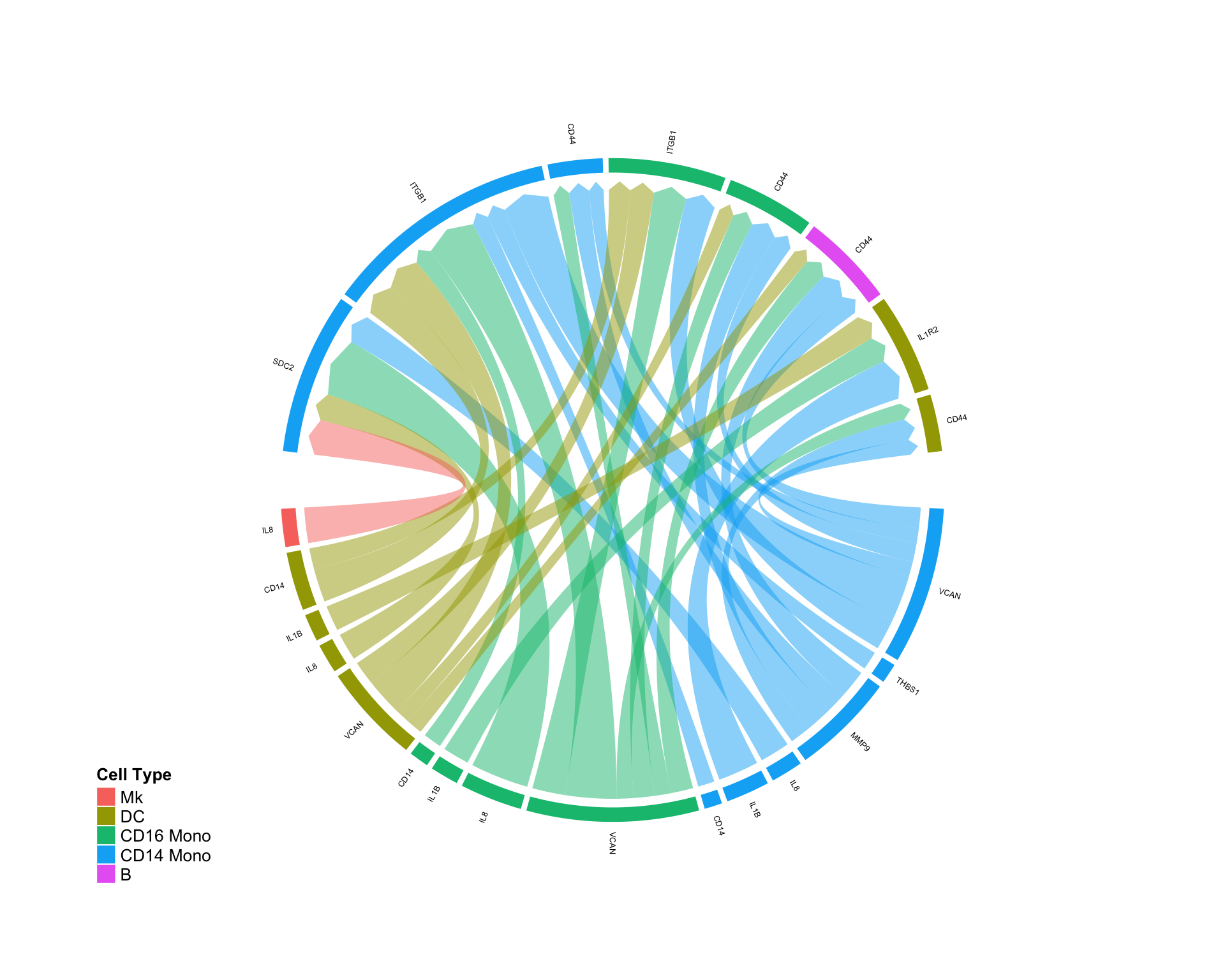
Quantifing pertubations in a cellular ‘niche’…

By subsetting to only those edges falling on a specific cell type, we can quantify the effect of a systemic perturbation (in this specific case, interferon treatment) on a given cellular niche:

CircosDiff(diff.sub,min.score = 2,min.pct = 0.1,lab.cex = 0.4,
           targets.include = c('CD14 Mono'))

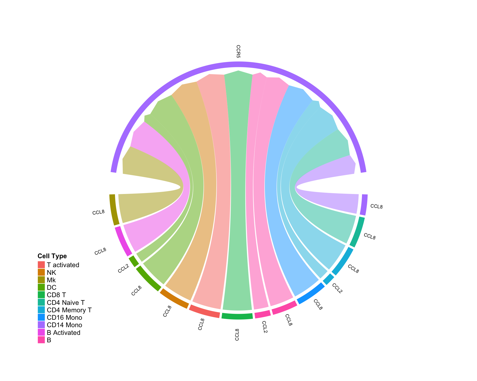
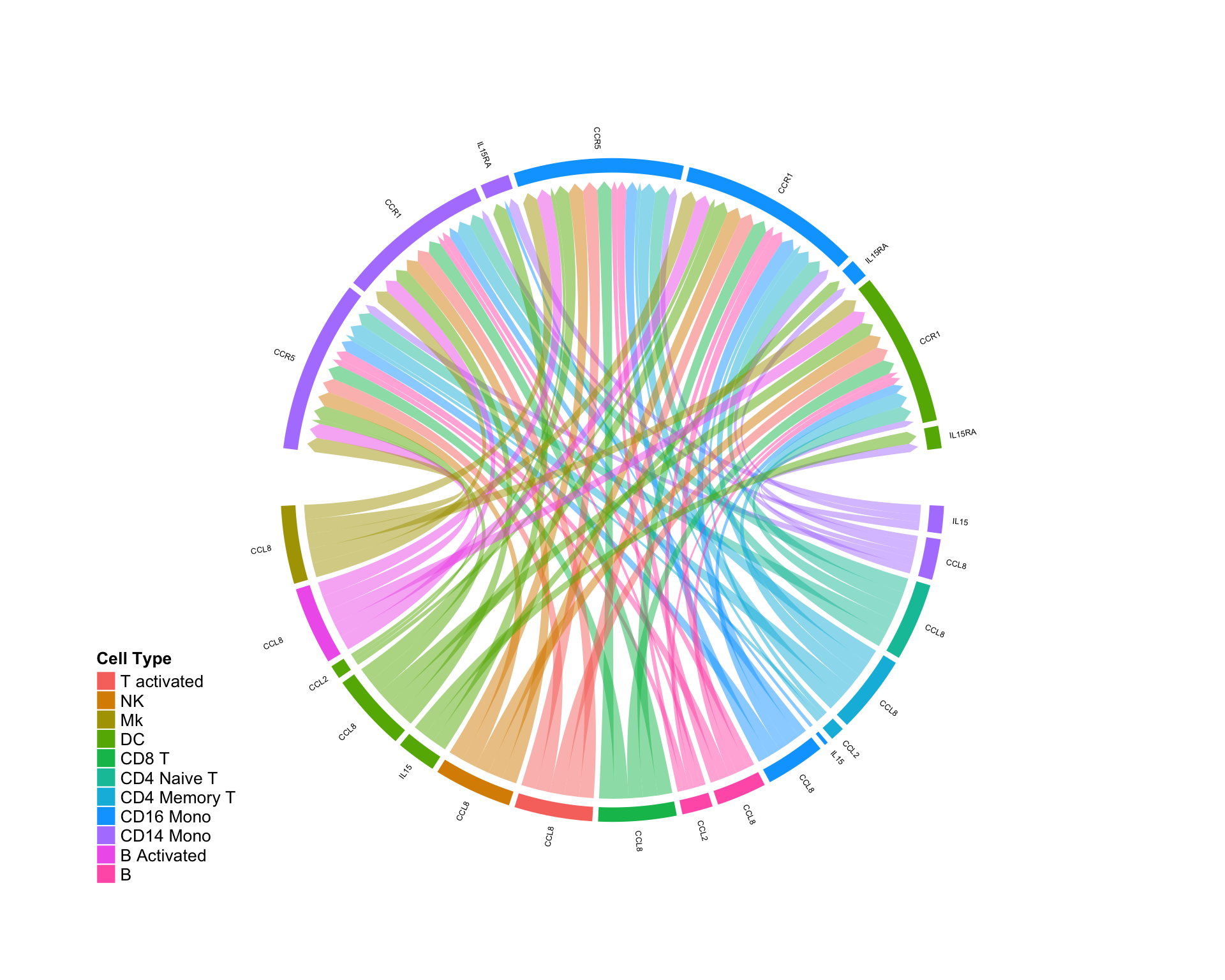
..or on a single receptor on a specific cell type

Since the above plot is still somehwat complex, we can further focus on the network landing on a single receptor, on a single cell type:

CircosDiff(diff.sub,min.score = 2,min.pct = 0.1,lab.cex = 0.6,
           targets.include = c('CD14 Mono'),features = c('CCR5'))

Differential Connectomics

Micha Sam Brickman Raredon

2020-05-13