Estimating Microenvironment from Spatial Data

NICHES is a toolset which transforms single-cell atlases into single-cell-signaling atlases. It is engineered to be computationally efficient and very easy to run. It interfaces directly with Seurat from Satija Lab. The cell-signaling outputs from NICHES may be analyzed with any single-cell toolset, including Seurat, Scanpy, Monocle, or others.

Here, we show how NICHES may be used to estimate individual cellular microenvironment from spatial transcriptomic data.

First, let’s load dependencies.

Load Dependencies

library(Seurat)
library(SeuratData)
library(ggplot2)
library(cowplot)
library(patchwork)
library(dplyr)
library(SeuratWrappers)
library(NICHES)
library(viridis)

Next, we load the data, perform basic pre-processing, and cluster the data so that we can visualize patterns of interest. For this vignette we will use basic Seurat clustering annotations to avoid the work of labeling celltypes, which are not necessary for this demonstration.

Load Data, Normalize, Visualize

InstallData("stxBrain")
brain <- LoadData("stxBrain", type = "anterior1")
# Normalization 
brain <- SCTransform(brain, assay = "Spatial", verbose = FALSE)
SpatialFeaturePlot(brain, features = c("Hpca", "Ttr"))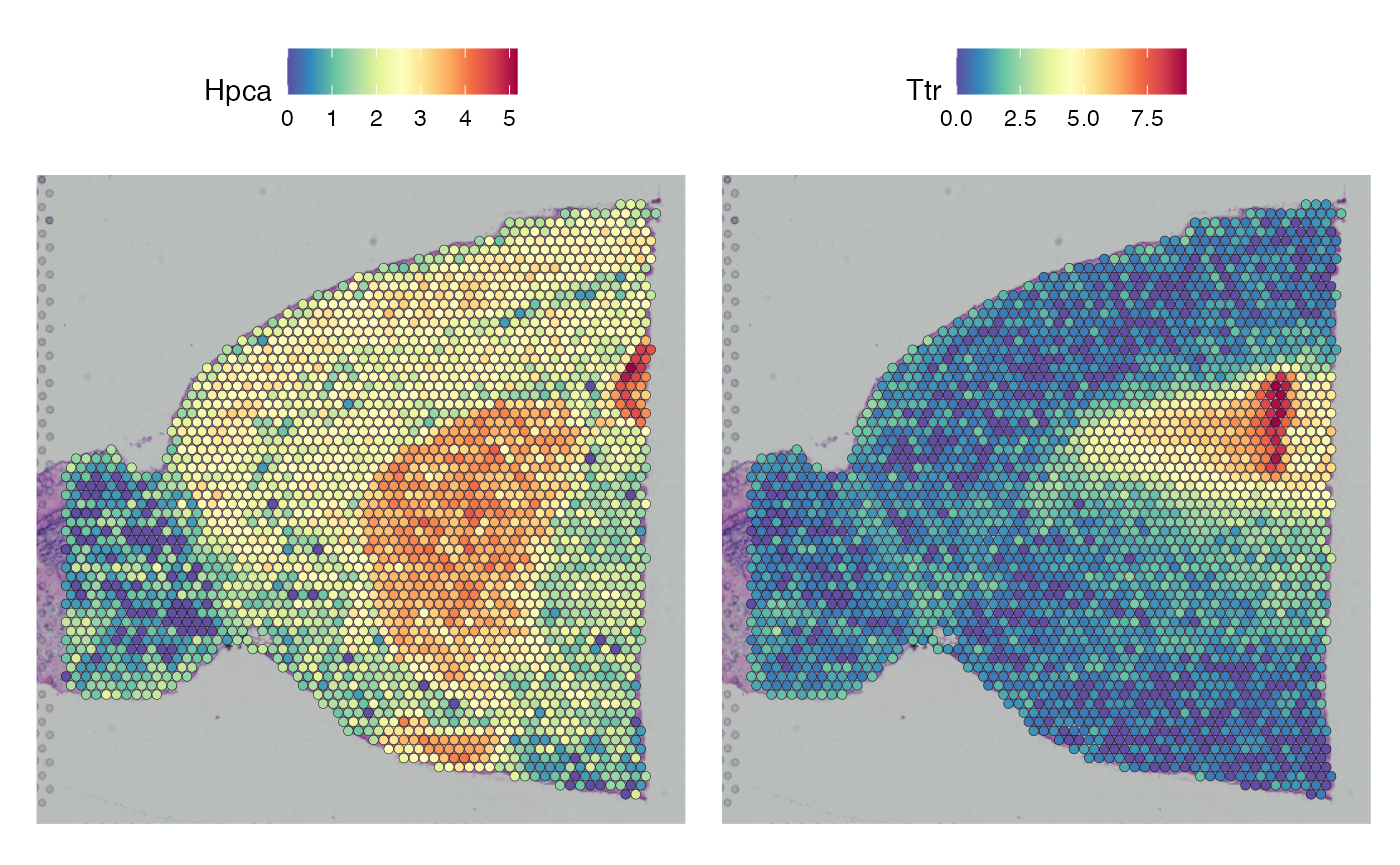

# Dimensional reduction with all cells
brain <- RunPCA(brain, assay = "SCT", verbose = FALSE)
brain <- FindNeighbors(brain, reduction = "pca", dims = 1:30)
brain <- FindClusters(brain, verbose = FALSE)
brain <- RunUMAP(brain, reduction = "pca", dims = 1:30)
p1 <- DimPlot(brain, reduction = "umap",group.by = 'seurat_clusters', label = TRUE)
p2 <- SpatialDimPlot(brain, label = TRUE,group.by = 'seurat_clusters', label.size = 3)
p1 + p2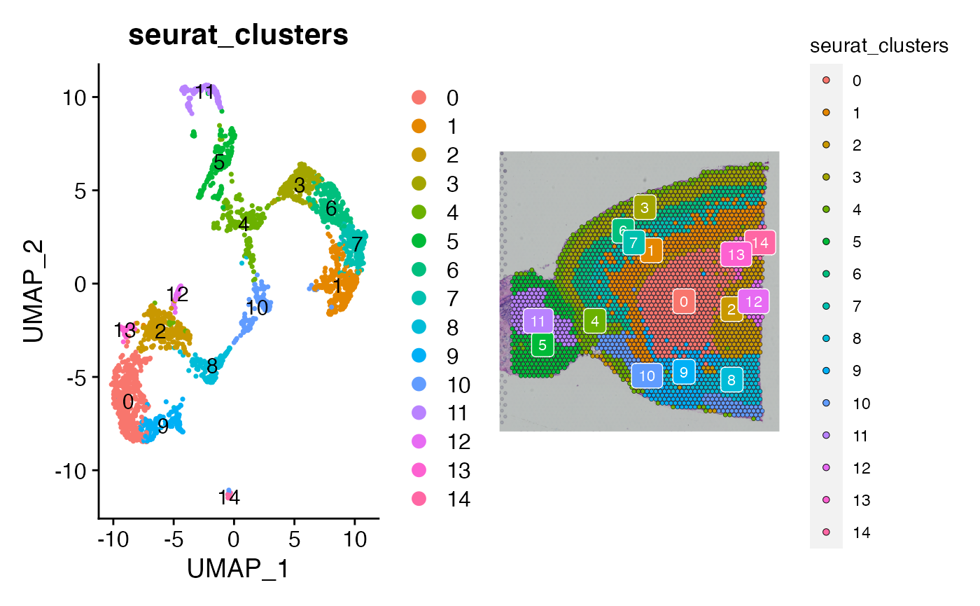

These numeric annotations are satisfactory for the demonstration of NICHES. Any and all metadata can be carried over when NICHES is run, allowing multiple levels of clustering and sub-clustering to be leveraged downstream after micorenvironment calculation.

Next, we will format the spatial coordinate metadata so that every cell has an explicitly labeled x and y coordinate.

Format Spatial Coordinates and Normalize

brain@meta.data$x <- brain@images$anterior1@coordinates$row
brain@meta.data$y <- brain@images$anterior1@coordinates$col

DefaultAssay(brain) <- "Spatial"
brain <- NormalizeData(brain)

NICHES can be run on imputed or non-imputed data. Here, we will use imputed data.

Impute and Run NICHES

brain <- SeuratWrappers::RunALRA(brain)

NICHES_output <- RunNICHES(object = brain,
                           LR.database = "fantom5",
                           species = "mouse",
                           assay = "alra",
                           position.x = 'x',
                           position.y = 'y',
                           k = 4, 
                           cell_types = "seurat_clusters",
                           min.cells.per.ident = 0,
                           min.cells.per.gene = NULL,
                           meta.data.to.map = c('orig.ident','seurat_clusters'),
                           CellToCell = F,CellToSystem = F,SystemToCell = F,
                           CellToCellSpatial = F,CellToNeighborhood = F,NeighborhoodToCell = T)

NICHES outputs a list of objects. Each object contains a certain style of cell-system signaling atlas. Above, we have only calculated a single one of interest, namely, individual cellular microenvironment. We next isolate this output and embed using UMAP to visualize the microenvironemnt of each cell.

niche <- NICHES_output[['NeighborhoodToCell']]
Idents(niche) <- niche[['ReceivingType']]

# Scale and visualize
niche <- ScaleData(niche)
niche <- FindVariableFeatures(niche,selection.method = "disp")
niche <- RunPCA(niche)
ElbowPlot(niche,ndims = 50)

niche <- RunUMAP(niche,dims = 1:10)
DimPlot(niche,reduction = 'umap',pt.size = 0.5,shuffle = T, label = T) +ggtitle('Cellular Microenvironment')+NoLegend()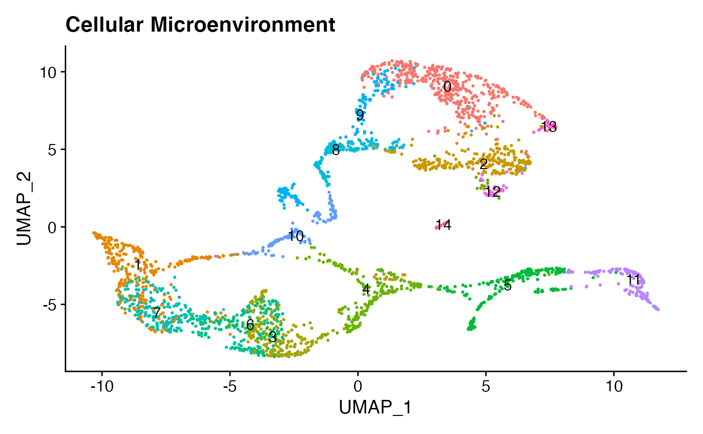

We can already see, from this plot, some notable overlap between the microenvironments of celltypes 1 & 7 and celltypes 6 & 3. Let’s explore this more deeply by finding signaling mechanisms specific to each celltype niche, plotting some of the results in heatmap form:

# Find markers
mark <- FindAllMarkers(niche,min.pct = 0.25,only.pos = T,test.use = "roc")
GOI_niche <- mark %>% group_by(cluster) %>% top_n(5,myAUC)
DoHeatmap(niche,features = unique(GOI_niche$gene))+ 
  scale_fill_gradientn(colors = c("grey","white", "blue"))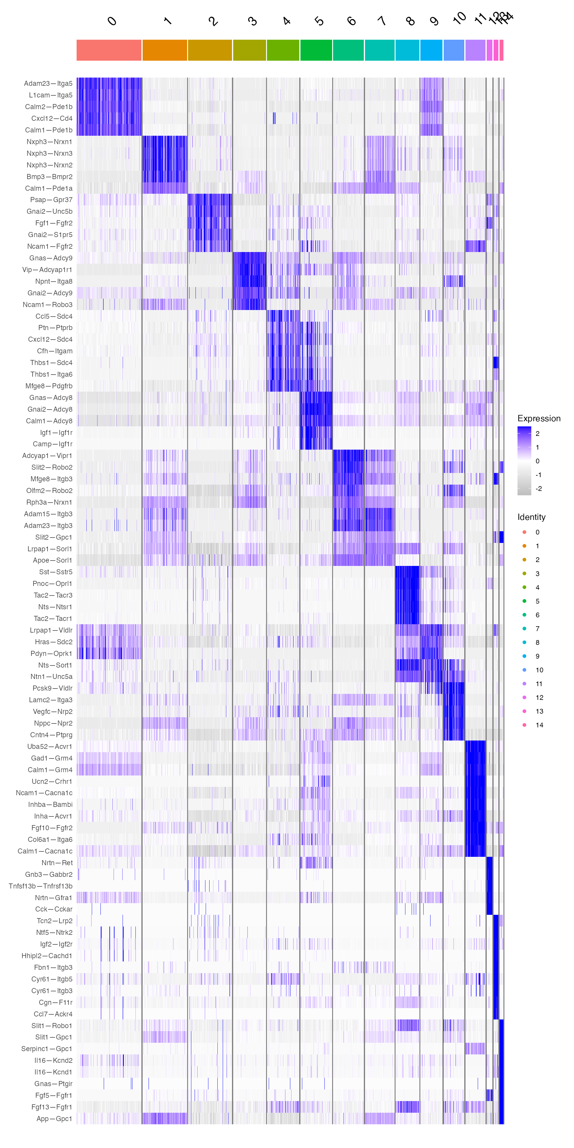

This confirms that celltypes 1 & 7 and 6 & 3 do indeed have some shared character.

We can further confirm that identified celltype specific signaling mechanisms are indeed specific to tissue regions in which those cells are found, by plotting matched ligand and receptor pairs:


# Check that these make sense and print little plots
DefaultAssay(brain) <- 'alra'
p1 <- SpatialFeaturePlot(brain, crop = TRUE, features = "Fgf1",slot = "data",min.cutoff =  'q1',
                         max.cutoff = 'q99')+ggtitle("Ligand")+theme(legend.position = "right")
p2 <- SpatialFeaturePlot(brain, crop = TRUE, features = "Fgfr2",slot = "data",min.cutoff =  'q1',
                         max.cutoff = 'q99')+ggtitle("Receptor")+theme(legend.position = "right")

ggpubr::ggarrange(p1,p2)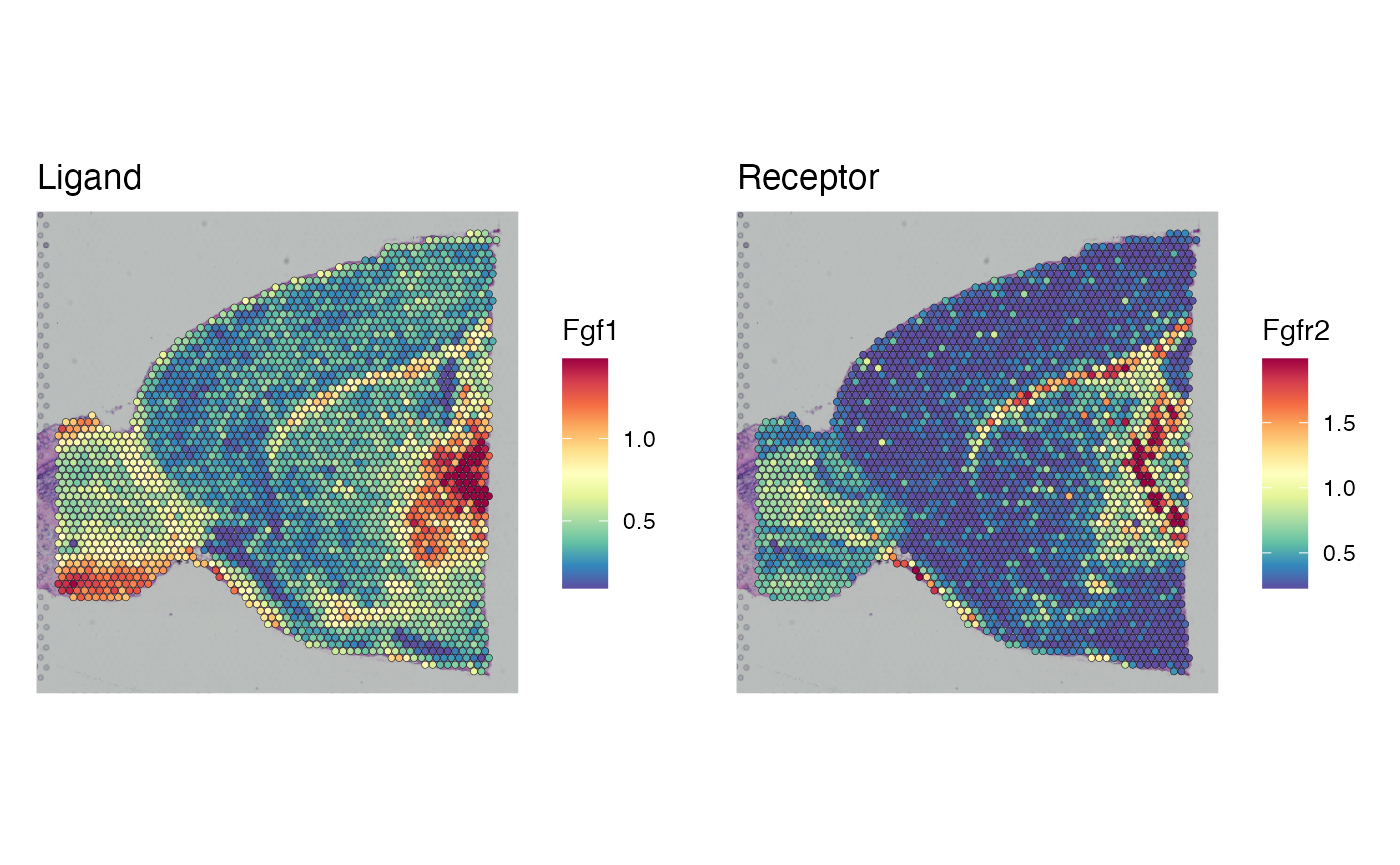

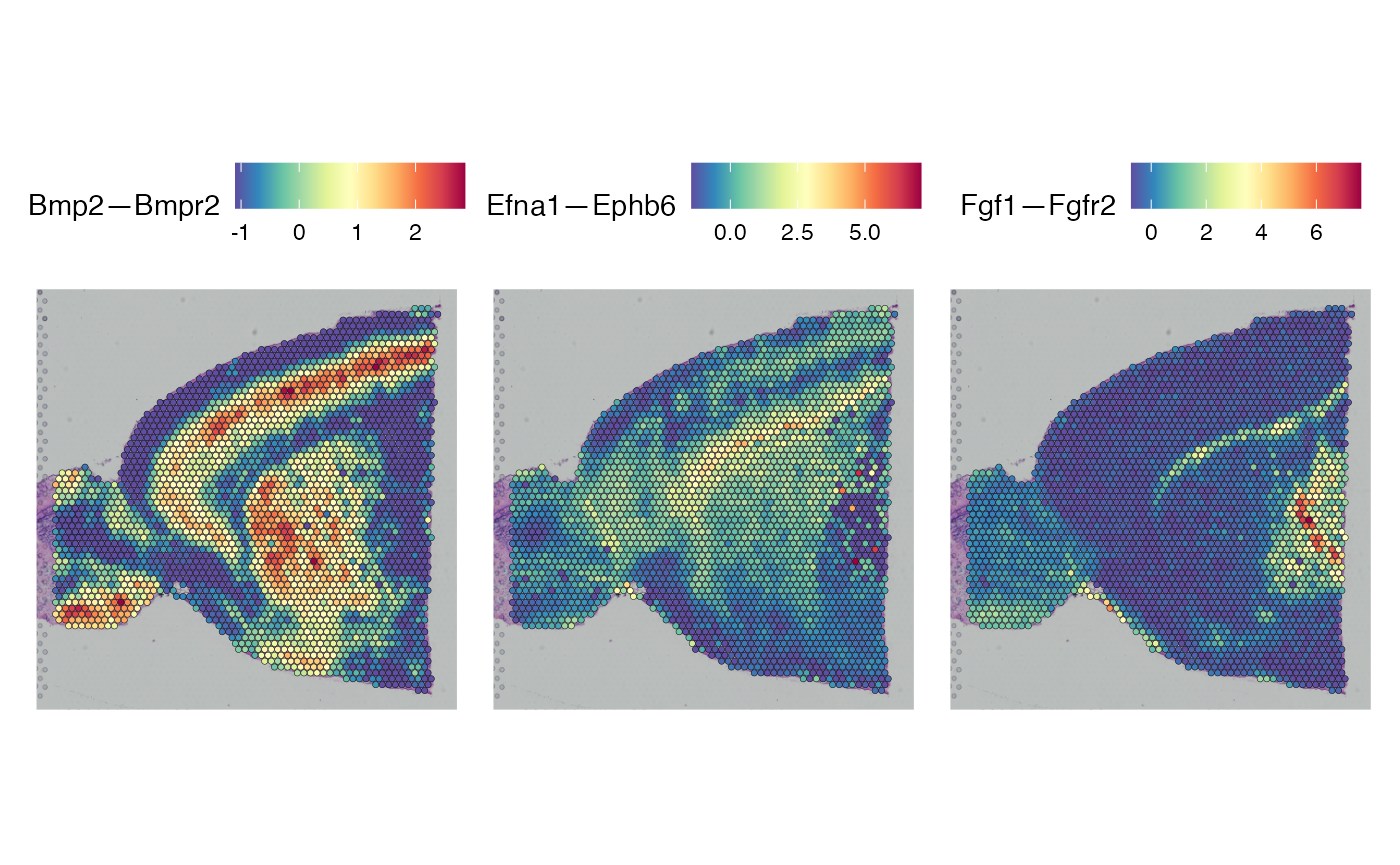
Further, and perhaps more usefully, we can map over the output from NICHES onto the original spatial object as follows:

# Add Niches output as an assay
niches.data <- GetAssayData(object =  niche[['NeighborhoodToCell']], slot = 'data')
colnames(niches.data) <- niche[['ReceivingCell']]$ReceivingCell
brain[["NeighborhoodToCell"]] <- CreateAssayObject(data = niches.data )
DefaultAssay(brain) <- "NeighborhoodToCell"
brain <- ScaleData(brain)

Which allows direct visualization of niche interactions of interest in a spatial context:

# Plot celltype specific niche signaling
SpatialFeaturePlot(brain,
                   features = c('Bmp2—Bmpr2','Efna1—Ephb6','Fgf1—Fgfr2'),
                   slot = 'scale.data')

Junchen Yang & Micha Sam Brickman Raredon

2022-07-20

Load Dependencies

Load Data, Normalize, Visualize

Format Spatial Coordinates and Normalize

Impute and Run NICHES