Interoperability

Junchen Yang

2022-07-20

In the previous vignettes, NICHES was mainly demonstrated with Seurat framework. Here in this vignette, we demonstrate the interoperability of NICHES with other popular scRNA-seq frameworks, namely, Scanpy, Monocle3, and scater.

First, let’s start with Scanpy and use the pbmc3k dataset as a demonstration. Scanpy is python-based and uses AnnData as the primary data strcture. We will demonstrate how to extract the data from Scanpy to run NICHES, convert the NICHES output to AnnData, and use functions from Scanpy to perform downstream analysis.

Interperobility with Scanpy

Load Required Packages

Here besides NICHES, we will also load ALRA for imputation and reticulate for running python.

library(NICHES)

# Load ALRA
devtools::source_url('https://raw.githubusercontent.com/KlugerLab/ALRA/master/alra.R')

# Set up reticulate and the python env
library(reticulate)
# change to your corresponding python path
Sys.setenv(RETICULATE_PYTHON = "/Library/Frameworks/Python.framework/Versions/3.10/bin/python3.10")

We will also need a few python packages, in particular, scanpy.

import numpy as np
import matplotlib.pyplot as plt
import scanpy as sc

sc.set_figure_params(dpi=300,figsize=(20,16))

Load the data and preprocess

Now let’s load the pbmc3k data from scanpy directly. Here we load both the raw and processed pbmc3k. The former will be used to run NICHES after a few processing steps and we will use the latter to add cell annotations.

# load the raw pbmc3k and the processed pbmc3k
adata = sc.datasets.pbmc3k()
#> WARNING: Failed to open the url with default certificates, trying with certifi.
#> 
  0%|          | 0.00/5.58M [00:00<?, ?B/s]
  1%|          | 32.0k/5.58M [00:00<00:28, 203kB/s]
  2%|1         | 88.0k/5.58M [00:00<00:17, 329kB/s]
  3%|3         | 192k/5.58M [00:00<00:20, 278kB/s] 
  7%|6         | 384k/5.58M [00:00<00:09, 547kB/s]
  8%|8         | 480k/5.58M [00:00<00:08, 618kB/s]
 11%|#         | 624k/5.58M [00:01<00:07, 681kB/s]
 12%|#2        | 688k/5.58M [00:01<00:07, 669kB/s]
 16%|#5        | 896k/5.58M [00:01<00:05, 874kB/s]
 21%|##        | 1.17M/5.58M [00:01<00:03, 1.35MB/s]
 23%|##3       | 1.29M/5.58M [00:01<00:03, 1.30MB/s]
 25%|##5       | 1.42M/5.58M [00:01<00:03, 1.25MB/s]
 28%|##8       | 1.57M/5.58M [00:01<00:03, 1.24MB/s]
 31%|###       | 1.71M/5.58M [00:02<00:03, 1.21MB/s]
 33%|###3      | 1.86M/5.58M [00:02<00:03, 1.21MB/s]
 36%|###5      | 2.01M/5.58M [00:02<00:03, 1.21MB/s]
 39%|###8      | 2.16M/5.58M [00:02<00:02, 1.23MB/s]
 41%|####1     | 2.31M/5.58M [00:02<00:02, 1.23MB/s]
 44%|####4     | 2.48M/5.58M [00:02<00:02, 1.25MB/s]
 47%|####7     | 2.62M/5.58M [00:02<00:02, 1.24MB/s]
 50%|####9     | 2.77M/5.58M [00:02<00:02, 1.30MB/s]
 51%|#####1    | 2.88M/5.58M [00:03<00:02, 1.22MB/s]
 53%|#####3    | 2.96M/5.58M [00:03<00:02, 1.10MB/s]
 56%|#####6    | 3.13M/5.58M [00:03<00:02, 1.15MB/s]
 58%|#####7    | 3.23M/5.58M [00:03<00:02, 1.10MB/s]
 60%|######    | 3.35M/5.58M [00:03<00:02, 990kB/s] 
 63%|######3   | 3.52M/5.58M [00:03<00:01, 1.11MB/s]
 66%|######5   | 3.68M/5.58M [00:03<00:02, 896kB/s] 
 69%|######8   | 3.85M/5.58M [00:04<00:01, 998kB/s]
 71%|#######   | 3.95M/5.58M [00:04<00:01, 880kB/s]
 71%|#######1  | 3.99M/5.58M [00:04<00:02, 780kB/s]
 75%|#######5  | 4.21M/5.58M [00:04<00:01, 1.07MB/s]
 77%|#######7  | 4.32M/5.58M [00:04<00:01, 1.03MB/s]
 80%|#######9  | 4.45M/5.58M [00:05<00:01, 618kB/s] 
 82%|########1 | 4.57M/5.58M [00:05<00:01, 678kB/s]
 84%|########4 | 4.70M/5.58M [00:05<00:01, 710kB/s]
 84%|########4 | 4.71M/5.58M [00:05<00:01, 606kB/s]
 88%|########8 | 4.92M/5.58M [00:05<00:00, 890kB/s]
 90%|########9 | 5.02M/5.58M [00:05<00:01, 565kB/s]
 92%|#########1| 5.13M/5.58M [00:06<00:00, 624kB/s]
 94%|#########3| 5.23M/5.58M [00:06<00:00, 676kB/s]
 96%|#########5| 5.34M/5.58M [00:06<00:00, 715kB/s]
 98%|#########7| 5.45M/5.58M [00:06<00:00, 750kB/s]
100%|#########9| 5.56M/5.58M [00:06<00:00, 761kB/s]
100%|##########| 5.58M/5.58M [00:06<00:00, 886kB/s]
adata2 = sc.datasets.pbmc3k_processed()
#> WARNING: Failed to open the url with default certificates, trying with certifi.
#> 
  0%|          | 0.00/23.5M [00:00<?, ?B/s]
  1%|          | 136k/23.5M [00:00<00:18, 1.34MB/s]
  2%|1         | 368k/23.5M [00:00<00:13, 1.80MB/s]
  3%|2         | 640k/23.5M [00:00<00:11, 2.14MB/s]
  4%|4         | 968k/23.5M [00:00<00:09, 2.57MB/s]
  5%|5         | 1.24M/23.5M [00:00<00:09, 2.43MB/s]
  7%|6         | 1.57M/23.5M [00:00<00:08, 2.71MB/s]
  8%|8         | 1.90M/23.5M [00:00<00:07, 2.88MB/s]
 10%|9         | 2.24M/23.5M [00:00<00:07, 3.07MB/s]
 11%|#         | 2.48M/23.5M [00:00<00:07, 2.88MB/s]
 12%|#2        | 2.88M/23.5M [00:01<00:06, 3.25MB/s]
 14%|#3        | 3.26M/23.5M [00:01<00:06, 3.44MB/s]
 15%|#5        | 3.55M/23.5M [00:01<00:06, 3.34MB/s]
 16%|#6        | 3.87M/23.5M [00:01<00:06, 3.28MB/s]
 18%|#7        | 4.21M/23.5M [00:01<00:06, 3.33MB/s]
 19%|#9        | 4.57M/23.5M [00:01<00:05, 3.43MB/s]
 21%|##        | 4.87M/23.5M [00:01<00:05, 3.33MB/s]
 22%|##2       | 5.21M/23.5M [00:01<00:05, 3.41MB/s]
 23%|##3       | 5.49M/23.5M [00:01<00:05, 3.25MB/s]
 25%|##4       | 5.85M/23.5M [00:02<00:05, 3.33MB/s]
 26%|##6       | 6.12M/23.5M [00:02<00:05, 3.14MB/s]
 28%|##7       | 6.48M/23.5M [00:02<00:05, 3.30MB/s]
 29%|##8       | 6.77M/23.5M [00:02<00:05, 3.15MB/s]
 30%|###       | 7.09M/23.5M [00:02<00:05, 3.17MB/s]
 31%|###1      | 7.37M/23.5M [00:02<00:05, 3.04MB/s]
 33%|###2      | 7.71M/23.5M [00:02<00:05, 3.19MB/s]
 34%|###4      | 8.01M/23.5M [00:02<00:05, 3.16MB/s]
 36%|###5      | 8.38M/23.5M [00:02<00:04, 3.38MB/s]
 37%|###7      | 8.73M/23.5M [00:02<00:04, 3.41MB/s]
 39%|###8      | 9.07M/23.5M [00:03<00:04, 3.46MB/s]
 40%|####      | 9.41M/23.5M [00:03<00:04, 3.49MB/s]
 42%|####1     | 9.77M/23.5M [00:03<00:04, 3.53MB/s]
 43%|####2     | 10.1M/23.5M [00:03<00:04, 3.49MB/s]
 44%|####4     | 10.4M/23.5M [00:03<00:04, 3.23MB/s]
 45%|####4     | 10.6M/23.5M [00:03<00:04, 2.77MB/s]
 46%|####5     | 10.8M/23.5M [00:03<00:05, 2.57MB/s]
 47%|####6     | 11.0M/23.5M [00:03<00:05, 2.52MB/s]
 48%|####7     | 11.2M/23.5M [00:03<00:05, 2.27MB/s]
 48%|####8     | 11.4M/23.5M [00:04<00:06, 2.09MB/s]
 49%|####9     | 11.6M/23.5M [00:04<00:05, 2.12MB/s]
 50%|#####     | 11.8M/23.5M [00:04<00:06, 1.98MB/s]
 51%|#####1    | 12.1M/23.5M [00:04<00:05, 2.28MB/s]
 53%|#####2    | 12.4M/23.5M [00:04<00:04, 2.61MB/s]
 54%|#####4    | 12.8M/23.5M [00:04<00:03, 2.93MB/s]
 56%|#####5    | 13.1M/23.5M [00:04<00:03, 3.08MB/s]
 57%|#####7    | 13.4M/23.5M [00:04<00:03, 3.16MB/s]
 59%|#####8    | 13.8M/23.5M [00:04<00:03, 3.31MB/s]
 60%|######    | 14.1M/23.5M [00:04<00:02, 3.39MB/s]
 62%|######1   | 14.5M/23.5M [00:05<00:02, 3.45MB/s]
 63%|######2   | 14.8M/23.5M [00:05<00:02, 3.28MB/s]
 64%|######4   | 15.1M/23.5M [00:05<00:02, 3.34MB/s]
 65%|######5   | 15.4M/23.5M [00:05<00:02, 3.22MB/s]
 67%|######6   | 15.7M/23.5M [00:05<00:02, 2.92MB/s]
 69%|######8   | 16.1M/23.5M [00:05<00:02, 3.38MB/s]
 70%|######9   | 16.4M/23.5M [00:05<00:02, 3.30MB/s]
 71%|#######1  | 16.7M/23.5M [00:05<00:02, 3.09MB/s]
 72%|#######2  | 17.0M/23.5M [00:05<00:02, 3.04MB/s]
 74%|#######3  | 17.3M/23.5M [00:05<00:02, 3.16MB/s]
 75%|#######5  | 17.7M/23.5M [00:06<00:01, 3.16MB/s]
 76%|#######6  | 17.9M/23.5M [00:06<00:01, 2.97MB/s]
 77%|#######7  | 18.2M/23.5M [00:06<00:01, 2.83MB/s]
 79%|#######8  | 18.5M/23.5M [00:06<00:01, 3.08MB/s]
 80%|########  | 18.9M/23.5M [00:06<00:01, 3.22MB/s]
 81%|########1 | 19.1M/23.5M [00:06<00:01, 3.12MB/s]
 83%|########2 | 19.5M/23.5M [00:06<00:01, 3.21MB/s]
 84%|########4 | 19.8M/23.5M [00:06<00:01, 3.06MB/s]
 85%|########5 | 20.0M/23.5M [00:06<00:01, 2.89MB/s]
 86%|########6 | 20.2M/23.5M [00:07<00:01, 2.62MB/s]
 87%|########6 | 20.4M/23.5M [00:07<00:01, 2.26MB/s]
 88%|########7 | 20.6M/23.5M [00:07<00:01, 2.24MB/s]
 88%|########8 | 20.8M/23.5M [00:07<00:01, 2.08MB/s]
 89%|########9 | 20.9M/23.5M [00:07<00:01, 1.92MB/s]
 90%|######### | 21.2M/23.5M [00:07<00:01, 2.01MB/s]
 91%|#########1| 21.5M/23.5M [00:07<00:00, 2.47MB/s]
 93%|#########2| 21.8M/23.5M [00:07<00:00, 2.74MB/s]
 94%|#########4| 22.2M/23.5M [00:07<00:00, 2.97MB/s]
 96%|#########5| 22.5M/23.5M [00:07<00:00, 3.10MB/s]
 97%|#########7| 22.9M/23.5M [00:08<00:00, 3.25MB/s]
 99%|#########8| 23.2M/23.5M [00:08<00:00, 3.33MB/s]
100%|#########9| 23.5M/23.5M [00:08<00:00, 3.12MB/s]
100%|##########| 23.5M/23.5M [00:08<00:00, 2.97MB/s]

# Filtering
sc.pp.filter_cells(adata, min_genes=200)
sc.pp.filter_genes(adata, min_cells=3)
adata.var['mt'] = adata.var_names.str.startswith('MT-')
sc.pp.calculate_qc_metrics(adata, qc_vars=['mt'], percent_top=None, log1p=False, inplace=True)
adata = adata[adata.obs.n_genes_by_counts < 2500, :]
adata = adata[adata.obs.pct_counts_mt < 5, :]
# Log1p normalization
sc.pp.normalize_total(adata, target_sum=1e4)
#> /Users/mbr29/Library/Python/3.10/lib/python/site-packages/scanpy/preprocessing/_normalization.py:170: UserWarning: Received a view of an AnnData. Making a copy.
#>   view_to_actual(adata)
sc.pp.log1p(adata)
# Assign labels
adata.obs['louvain'] = adata2.obs['louvain']

Visualize the data

We can visualize the processed data on UMAP using Scanpy.

with plt.rc_context({"figure.figsize": (8, 8), "figure.dpi": (300)}):
    sc.pl.umap(adata2, color='louvain',legend_loc ="on data")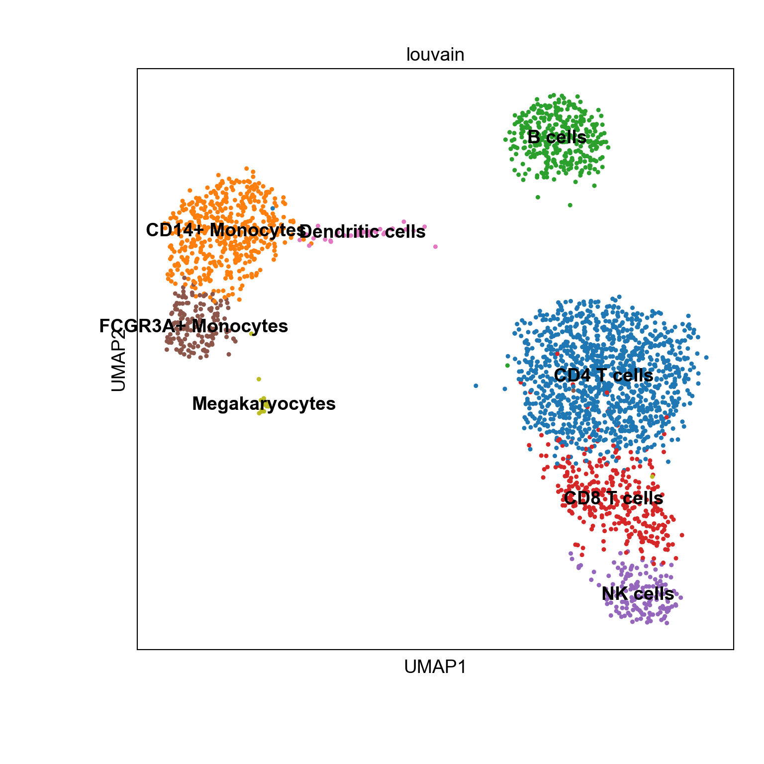

Subset to only ‘B cells’,‘CD4 T cells’,‘CD14+ Monocytes’

Here for demonstration, For let’s focus in on signaling within a simple 3-cell system:

adata = adata[adata.obs['louvain'].isin(['B cells','CD4 T cells','CD14+ Monocytes']),:]

cell_names = np.array(adata.obs_names)
gene_names = np.array(adata.var_names)

Extract the meta data and impute the data to run NICHES

Here we will extract the cell types metadata from anndata and impute the data to run NICHES. In particular, data.imputed will the data matrix to run NICHES.

meta.data.df <- data.frame("louvain" = py$adata$obs$louvain,row.names = py$cell_names)

# alra imputation
imputed.list <- alra(as.matrix(py$adata$X$toarray()))
#> Read matrix with 1966 cells and 13714 genes
#> Chose k=16
#> Getting nonzeros
#> Randomized SVD
#> Find the 0.001000 quantile of each gene
#> Sweep
#> Scaling all except for 393 columns
#> 0.00% of the values became negative in the scaling process and were set to zero
#> The matrix went from 5.89% nonzero to 40.75% nonzero
data.imputed <- t(imputed.list[[3]])

colnames(data.imputed) <- py$cell_names
rownames(data.imputed) <- py$gene_names

Run NICHES

Here we will take the previously imputed data matrix as input to run NICHES and specify output_format to be “raw” for easier conversion to AnnData.

niches_list <- RunNICHES(data.imputed,
                 meta.data.df = meta.data.df,
                 cell_types = "louvain",
                 species = 'human',
                 LR.database = 'fantom5',
                 CellToCell = T,output_format = "raw"
                 )
lr_names <- rownames(niches_list$CellToCell$CellToCellMatrix)

Convert the output to AnnData

We will extract the output CellToCellMatrix from NICHES and convert it to AnnData.

adata_niches = sc.AnnData(X = r.niches_list['CellToCell']['CellToCellMatrix'].T)
#> <string>:1: FutureWarning: X.dtype being converted to np.float32 from float64. In the next version of anndata (0.9) conversion will not be automatic. Pass dtype explicitly to avoid this warning. Pass `AnnData(X, dtype=X.dtype, ...)` to get the future behavour.
adata_niches.obs = r.niches_list['CellToCell']['metadata']
adata_niches.var_names = r.lr_names

Process the output from NICHES using Scanpy

We will use the Scanpy functions to perform downstream analysis. Here we will scale the data, do PCA and UMAP.

# data scaling, pca, find neighbors, and umap
sc.pp.scale(adata_niches)
sc.tl.pca(adata_niches)
sc.pp.neighbors(adata_niches)
sc.tl.umap(adata_niches)

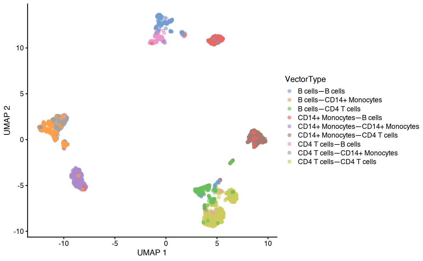
Visualize CellToCell matrix

We can use the visualization function from Scanpy to visualize the data in UMAP.

with plt.rc_context({"figure.figsize": (8, 8), "figure.dpi": (300)}):
    sc.pl.umap(adata_niches,color="VectorType",legend_loc ="on data",legend_fontsize=7)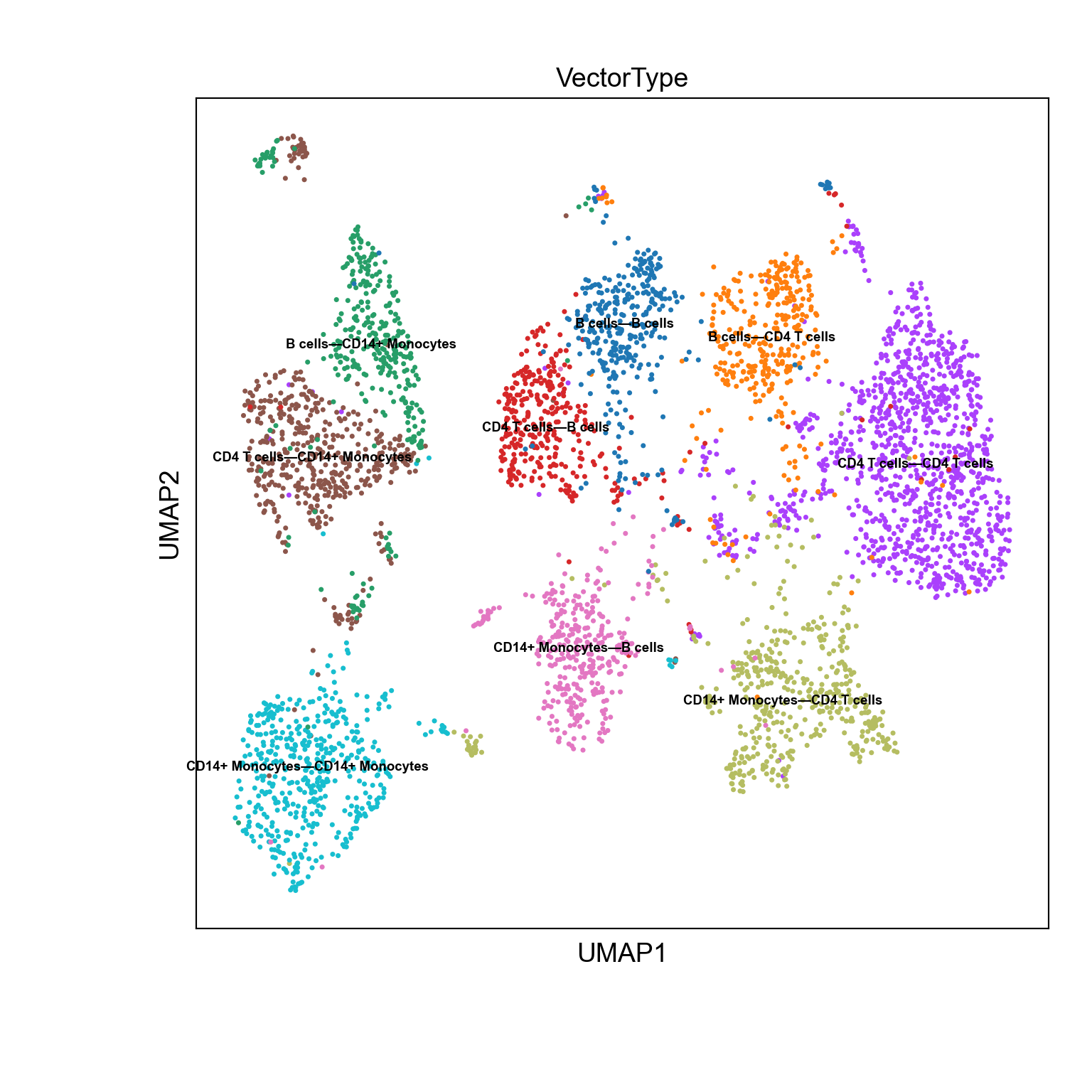

Differential analysis

We can also use the function from Scanpy to perform differential analysis between different VectorTypes. Here we will rank the genes using a logistic regression classifier with L1 regularization and visualize the top markers.

sc.tl.rank_genes_groups(adata_niches, 'VectorType', method='logreg', solver='liblinear',penalty='l1')
with plt.rc_context({"figure.figsize": (8, 12), "figure.dpi": (300)}):
    sc.pl.rank_genes_groups(adata_niches, n_genes=5, sharey=False,show=True,fontsize=20)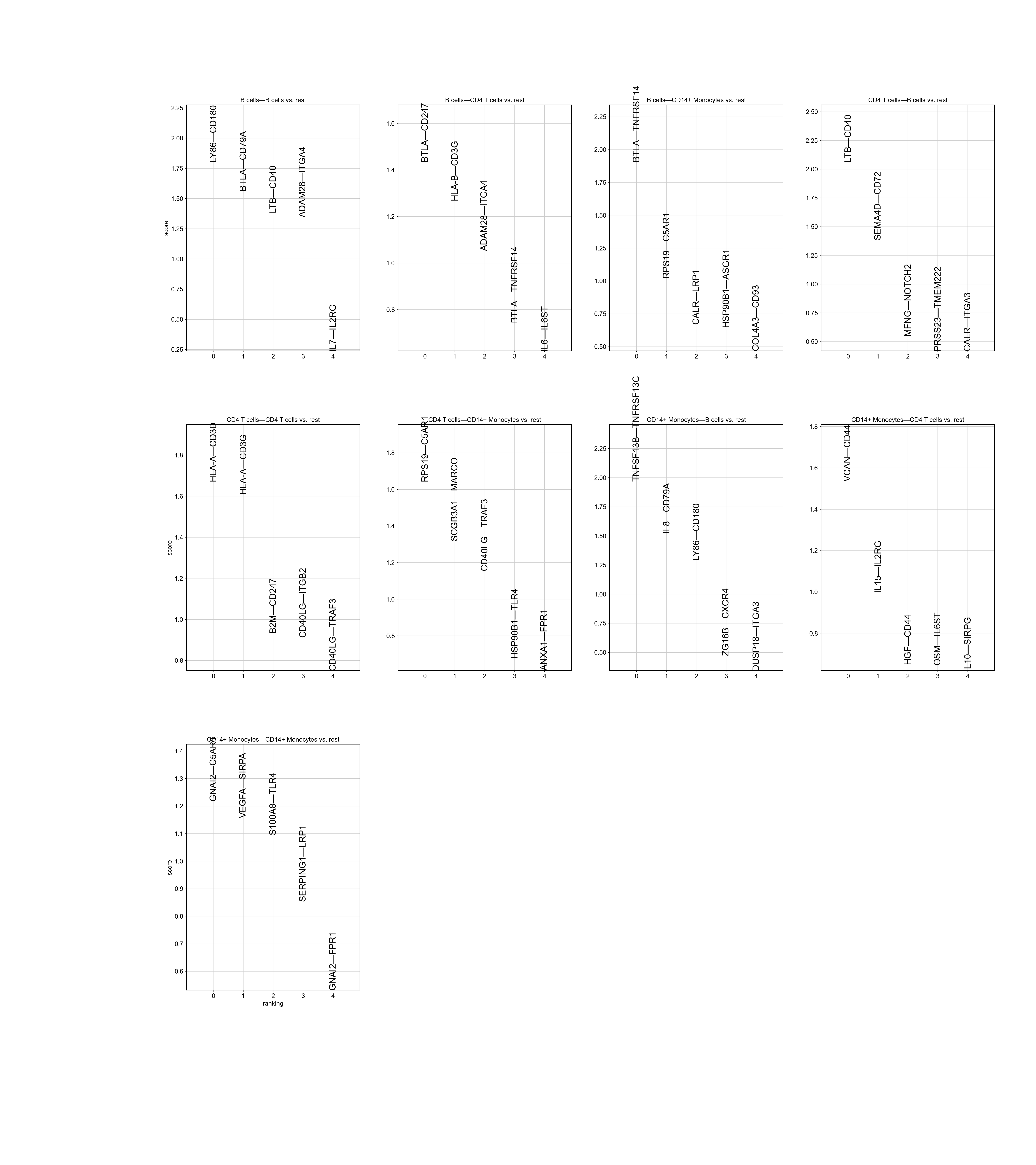

We can also check the interaction levels on violin plot for certain markers.

marker_LRs = np.array([g for g in adata_niches.uns['rank_genes_groups']['names'][0]])

# check specific LRs
with plt.rc_context({"figure.figsize": (10,7), "figure.dpi": (300),"font.size":(8)}):
    sc.pl.violin(adata_niches, marker_LRs[0], groupby='VectorType',rotation=20)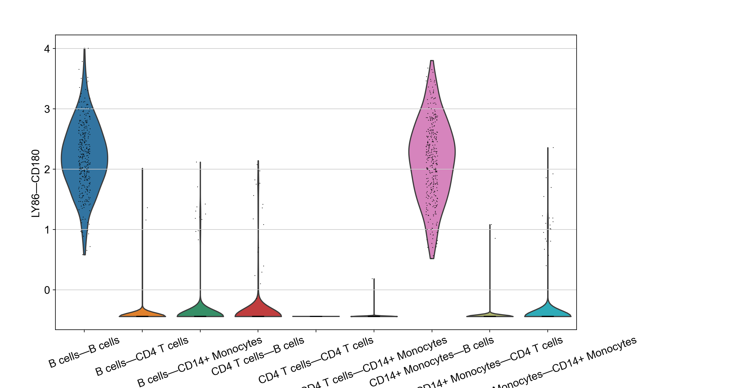

We can also visualize the interaction levels on top of UMAP.

with plt.rc_context({"figure.figsize": (8, 8), "figure.dpi": (300)}):
    sc.pl.umap(adata_niches, color=marker_LRs[:2],ncols=2)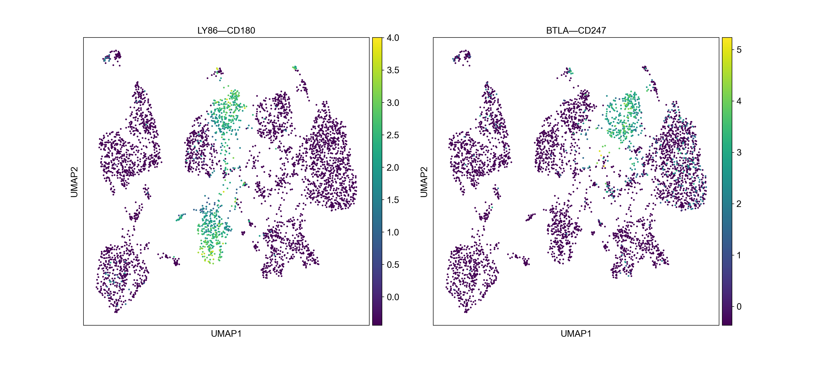

We can also visualize the interaction levels for the top markers of different groups using dot plot.

with plt.rc_context({"figure.dpi": (300),"font.size":(10)}):
    sc.pl.dotplot(adata_niches, marker_LRs, groupby='VectorType',figsize=(20,10))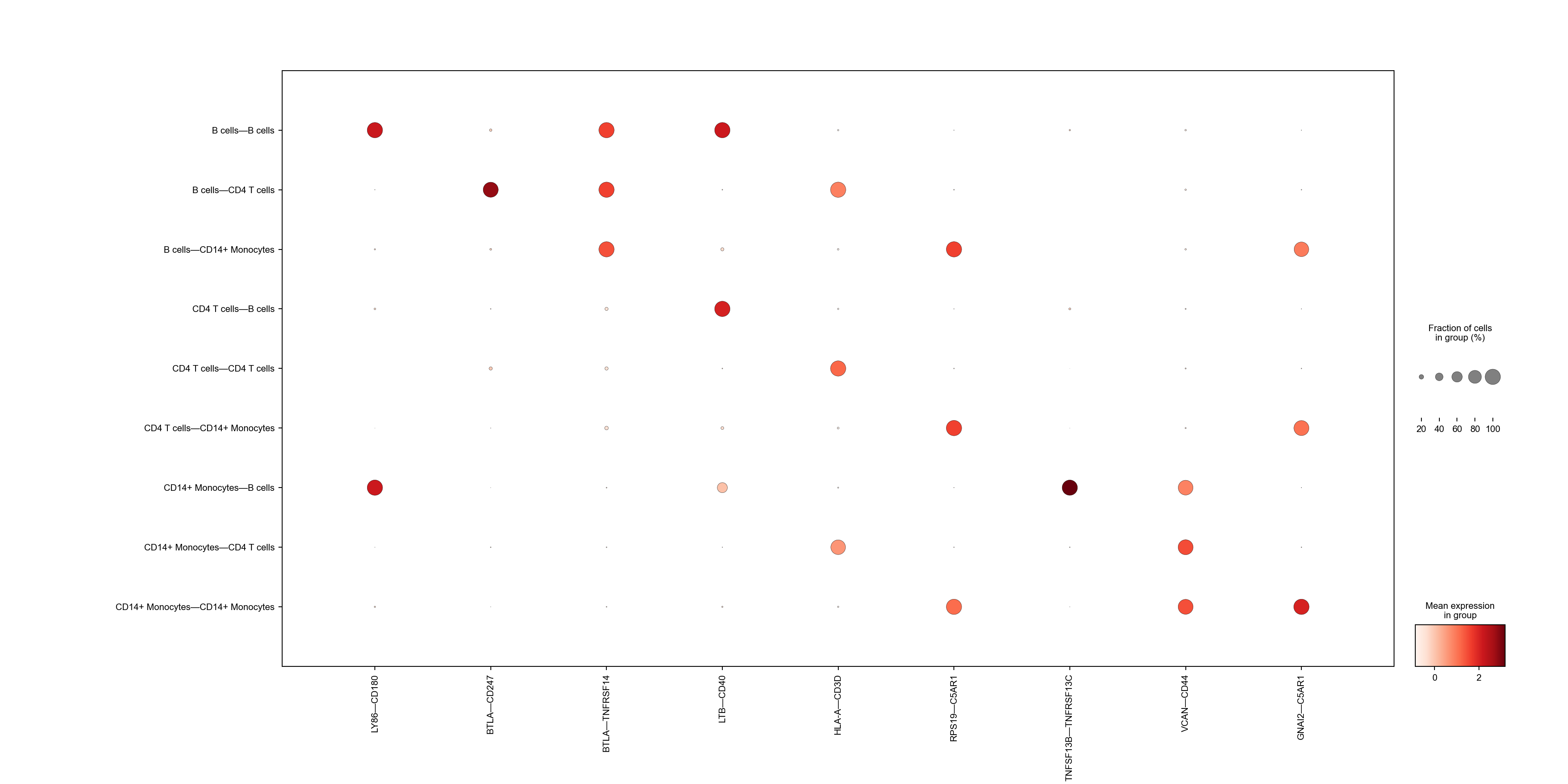

Interporability with Monocle3 (CellDataSet)

Here we will continue to use this pbmc3k dataset, but we will switch to Monocle3 (CellDataSet). This will be a simple demonstration of how to convert the output from NICHES to CellDataSet and use certain functions from Monocle3 to perform downstream analysis.

Convert the output from NICHES to CellDataSet

Here we use the same output from NICHES from previous run and convert it to CellDataSet.

library(monocle3)
lr_metadata <- data.frame(lr_names)
rownames(lr_metadata) <- lr_names
cds <- new_cell_data_set(niches_list$CellToCell$CellToCellMatrix,
                         cell_metadata = niches_list$CellToCell$metadata,
                         gene_metadata = lr_metadata)

Data Processing

Then we will process the data using Monocle3 and run PCA and UMAP on it.

# use all genes for pca
cds <- preprocess_cds(cds, num_dim = 30,
                      method = "PCA",norm_method = "none",scaling = TRUE,verbose = TRUE)

cds <- reduce_dimension(cds)

Data Visualization

We can visualize the data on UMAP (Cells are colored by VectorTypes).

plot_cells(cds, color_cells_by="VectorType")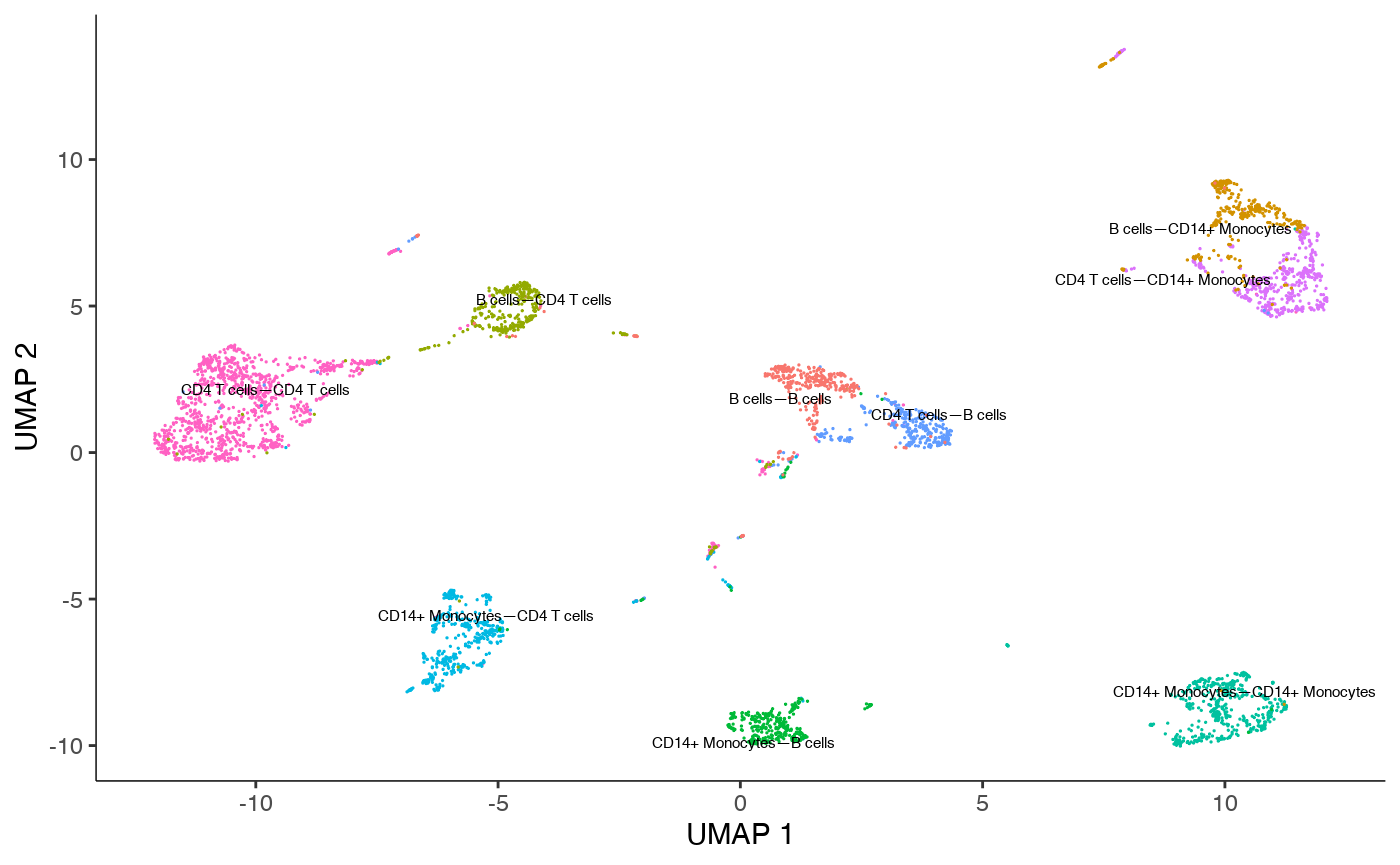

Interporability with Scater (SingleCellExperiment)

Here we will continue to use this pbmc3k dataset, but we will switch to Scater (SingleCellExperiment) and utilize certain functions to perform downstream analysis.

Convert the output from NICHES to SingleCellExperiment

library(scater)
sce <- SingleCellExperiment(
    assays = list(data = niches_list$CellToCell$CellToCellMatrix), 
    colData = niches_list$CellToCell$metadata,
    rowData = lr_metadata
)

RunPCA on the ouput

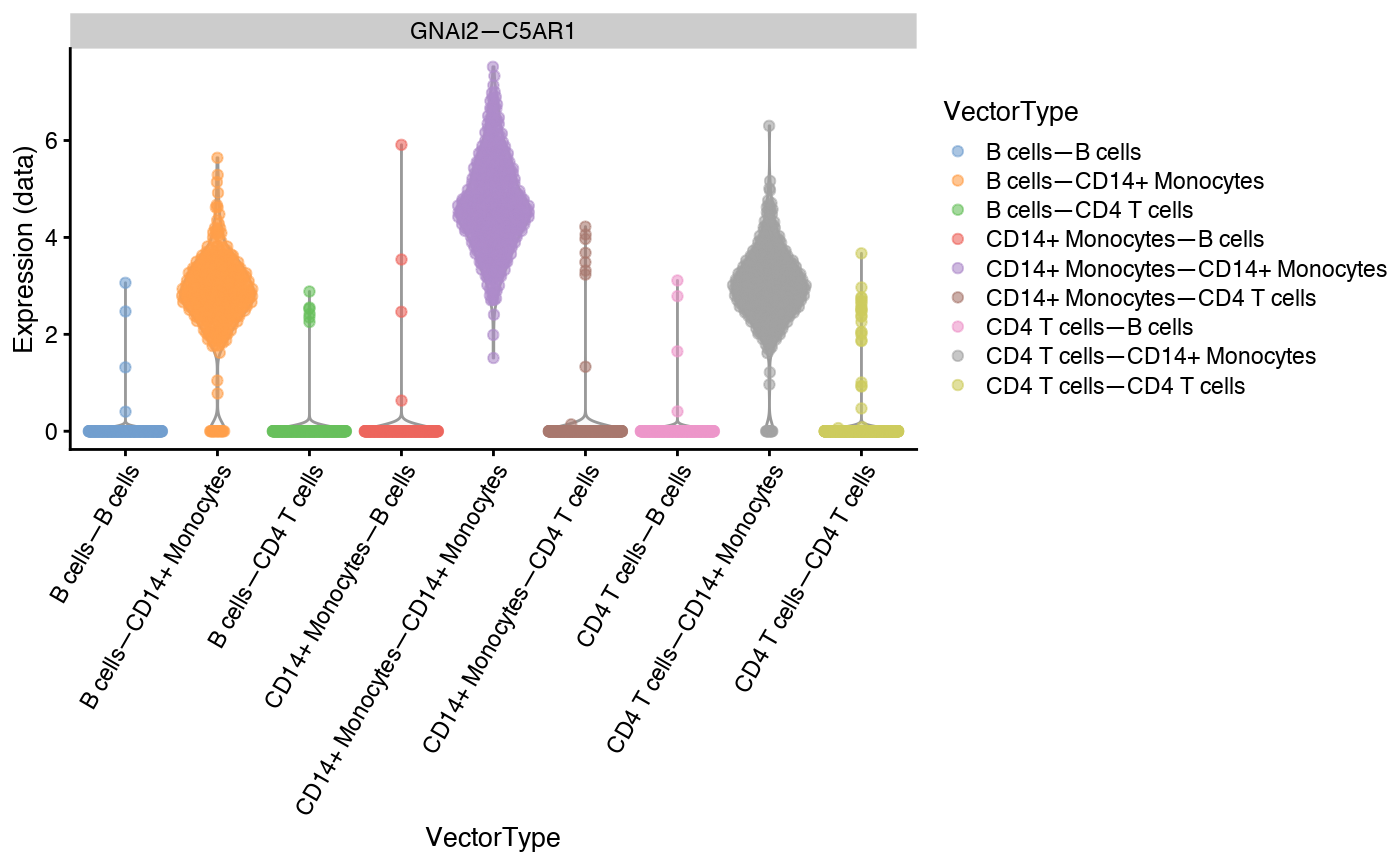
sce <- runPCA(sce,exprs_values="data")

Visualize Ligand-receptor interactions using violin plot

plotExpression(sce,features = "GNAI2—C5AR1",exprs_values = "data",x = "VectorType",colour_by="VectorType")+
  theme(axis.text.x = element_text(angle = 60, vjust = 1, hjust=1))

Visualize the output on UMAP

sce <- runUMAP(sce,exprs_values="data")

plotUMAP(sce, colour_by = "VectorType")