Differential CellToCell Signaling Across Conditions
Wes Lewis & Micha Sam Brickman Raredon
2022-07-20
04 Differential CellToCell.RmdA common question is how to use NICHES to assess differential signaling across experimental conditions or batches. This is a task that is exceptionally easy in NICHES if performed in the correct way. Here, we demonstrate how to approach this task, using the publicly available ‘ifnb’ dataset within SeuratData which allows comparision of IFNb-stimualted PBMCs versus control PBMCs.
Load Data and Explore Metadata
library(SeuratData)
#InstallData("ifnb")
data("ifnb")
table(ifnb@meta.data$stim,ifnb@meta.data$seurat_annotations)
#>
#>        CD14 Mono CD4 Naive T CD4 Memory T CD16 Mono    B CD8 T T activated   NK
#>   CTRL      2215         978          859       507  407   352         300  298
#>   STIM      2147        1526          903       537  571   462         333  321
#>
#>          DC B Activated   Mk  pDC Eryth
#>   CTRL  258         185  115   51    23
#>   STIM  214         203  121   81    32
This dataset contains two experimental conditions, annotated STIM and CTRL. Prior to running NICHES, we will split the dataset into two objects, one representing each experimental condition. This way, cells will only be crossed with cells in the same experimental condition.
Split by Experimental Contion
# Set idents so that celltypes are in active identity slot
Idents(ifnb) <- ifnb@meta.data["seurat_annotations"]
# Split object into STIM and CTRL conditions, to calculate NICHES objects separately
data.list <- SplitObject(ifnb, split.by="stim")
# Make sure that data is normalized
data.list <- lapply(X = data.list, FUN = function(x) {
    x <- NormalizeData(x)
})
We now are prepared to run NICHES separately on the cell systems present in each experimental condition.
Run NICHES
# Run NICHES on each system and store/name the outputs
scc.list <- list()
for(i in 1:length(data.list)){
  print(i)
  scc.list[[i]] <- RunNICHES(data.list[[i]],
                             LR.database="fantom5",
                             species="human",
                             assay="RNA",
                             cell_types = "seurat_annotations",
                             min.cells.per.ident=1,
                             min.cells.per.gene = 50,
                             meta.data.to.map = c('orig.ident','seurat_annotations','stim'),
                             SystemToCell = T,
                             CellToCell = T)
}
#> [1] 1
#> [1] 2
names(scc.list) <- names(data.list)
NICHES provides output as a list of objects or tables, because it is capable of providing many different styles of output with a single run. Let’s isolate a specific output style we are interested in and tag it with appropriate metadata (redundant here, but good practice)
Isolate Output of Interest
temp.list <- list()
for(i in 1:length(scc.list)){
temp.list[[i]] <- scc.list[[i]]$CellToCell # Isolate CellToCell Signaling, which is all that will be covered in this vignette
temp.list[[i]]$Condition <- names(scc.list)[i] # Tag with metadata
}
We can then merge these NICHES outputs together to embed, cluster, and analyze them jointly:
Merge and Clean
# Merge together
scc.merge <- merge(temp.list[[1]],temp.list[2])

# Clean up low-information crosses (connectivity data can be very sparse)
VlnPlot(scc.merge,features = 'nFeature_CellToCell',group.by = 'Condition',pt.size=0.1,log = T)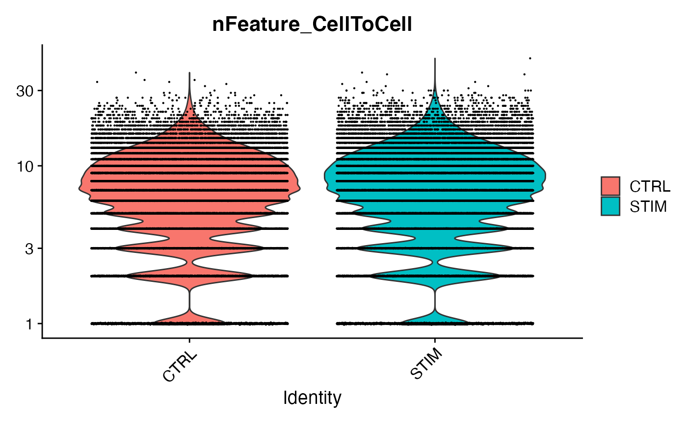
scc.sub <- subset(scc.merge,nFeature_CellToCell > 5) # Requesting at least 5 distinct ligand-receptor interactions between two cellsLet’s now perform an initial visualization of signaling between these two conditions, which we do as follows:
Visualize full dataset
# Perform initial visualization
scc.sub <- ScaleData(scc.sub)
scc.sub <- FindVariableFeatures(scc.sub,selection.method = "disp")
scc.sub <- RunPCA(scc.sub,npcs = 50)
ElbowPlot(scc.sub,ndim=50)
We choose to use the first 25 principle components for a first embedding:
DimPlot(scc.sub,group.by = 'Condition')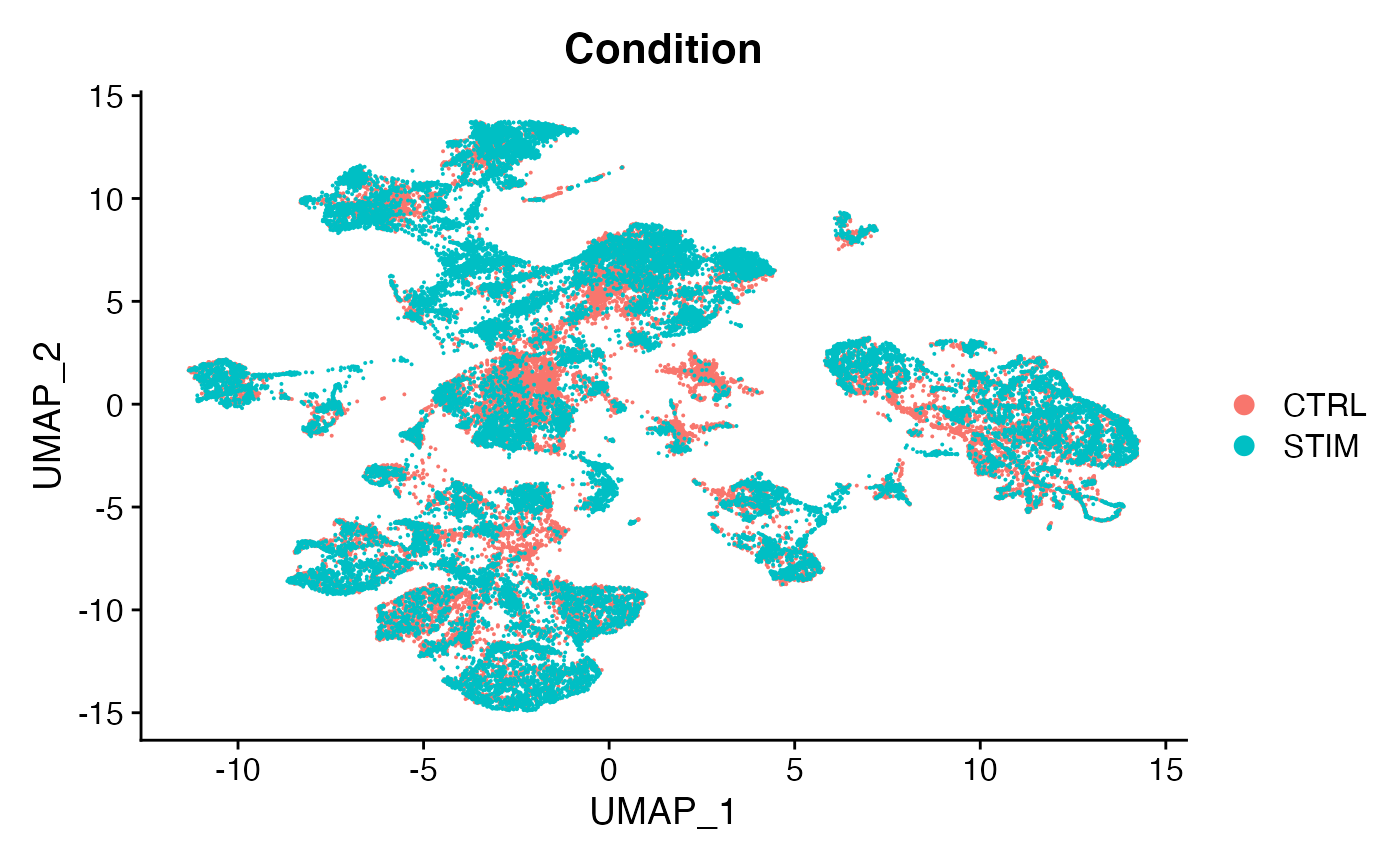
DimPlot(scc.sub,group.by = 'ReceivingType')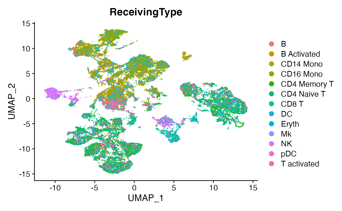
DimPlot(scc.sub,group.by = 'SendingType')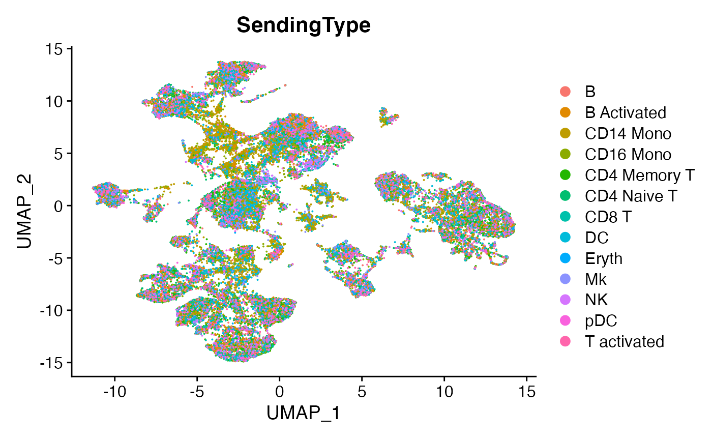
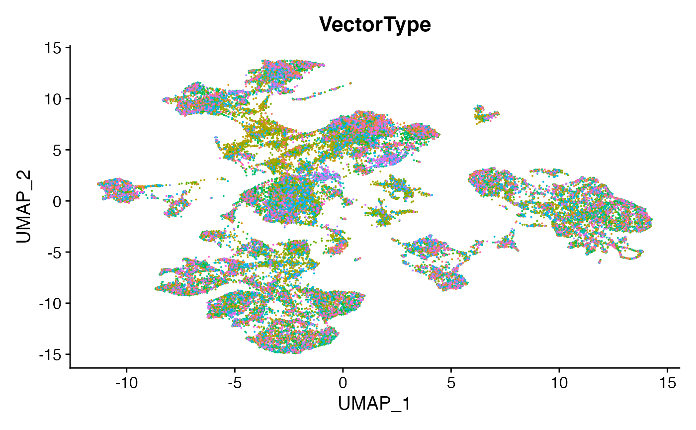
One thing we can do at this point is to ask how signaling is different between conditions for an individual cell-to-cell VectorType, which we do as follows:
Focus on a single cell-cell cross of interest
head(unique(scc.sub@meta.data$VectorType))
#> [1] "CD14 Mono—CD14 Mono"    "CD14 Mono—CD4 Naive T"  "CD14 Mono—CD4 Memory T"
#> [4] "CD14 Mono—CD16 Mono"    "CD14 Mono—B"            "CD14 Mono—CD8 T"
# Define VectorTypes of interest (note the long em-dash used in NICHES)
VOI <- "CD14 Mono—DC"
# Loop over VectorTypes of interest, subsetting those interactions, finding markers associated with the comparison of interest (stimulus vs control) and  create a heatmap of top markers:
lapply(VOI, function(x){

  #subset
  subs <- subset(scc.sub, subset = VectorType == x)

  #print number of cells per condition
  print(paste0(x , ":  CTRL:", sum(subs@meta.data$Condition == "CTRL")))
  print(paste0(x , ":  STIM:", sum(subs@meta.data$Condition == "STIM")))

  #set idents
  Idents(subs) <- subs@meta.data$Condition

  #scale the subsetted data
  FindVariableFeatures(subs,assay='CellToCell',selection.method = "disp")
  ScaleData(subs, assay='CellToCell')

  #these are the features in the scaledata slot
  feats <- dimnames(subs@assays$CellToCell@scale.data)[[1]]
  feats

  #find markers (here we use wilcox, but ROC and other tests can be used as well)
  markers <- FindAllMarkers(subs, features=feats, test.use = "wilcox",assay='CellToCell')

  #subset to top 10 markers per condition
  top10 <- markers %>% group_by(cluster) %>% top_n(n = 10, wt = avg_log2FC)

  #Make a heatmap
  DoHeatmap(subs,group.by="ident",features=top10$gene, assay="CellToCell") +  ggtitle("Top DE Mechanisms, CTRL vs STIM: ",x)
})
#> [1] "CD14 Mono—DC:  CTRL:216"
#> [1] "CD14 Mono—DC:  STIM:191"
#> [[1]]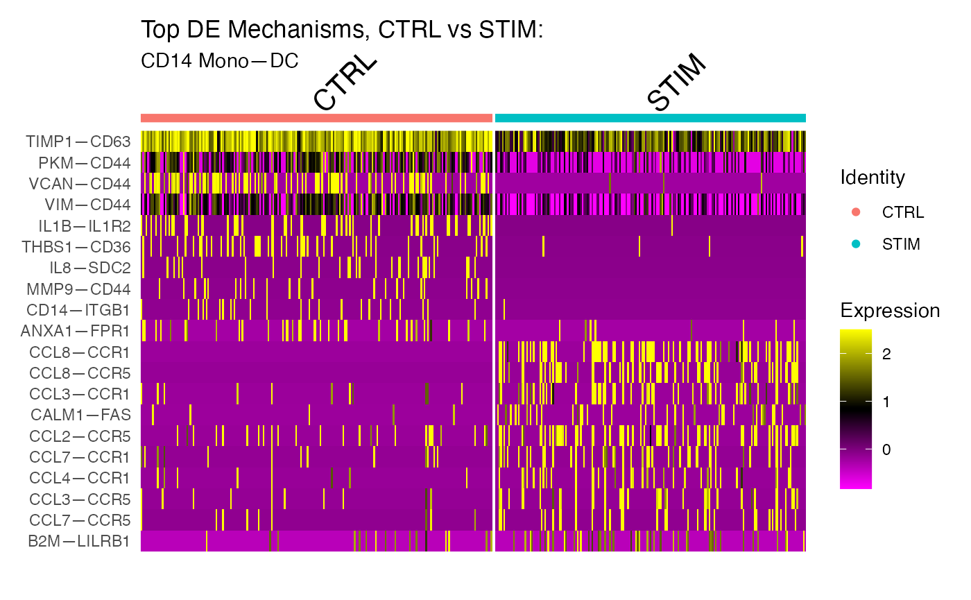
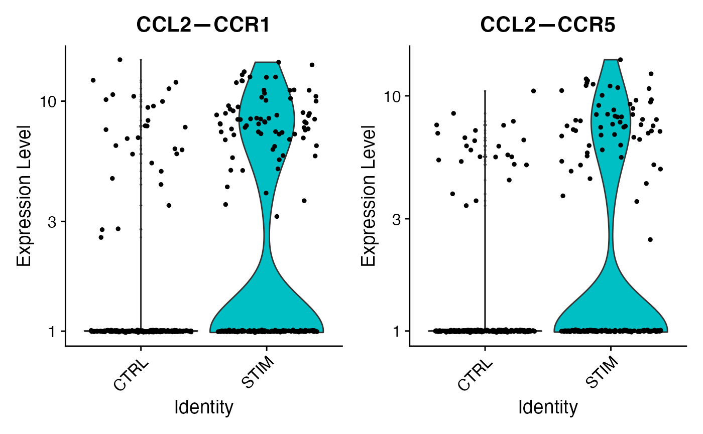
These results confirm our expectation that chemokine signaling for this cell-cell VectorType is upregulated in the STIM condition as compared to contol. We can further isolate this specific VectorType for embedding or clustering:
# Perform visualization for VectorTypes of interest
VOI <- c("CD14 Mono—DC")
Idents(scc.sub) <- scc.sub@meta.data$VectorType
voi.data <- subset(scc.sub,idents = VOI)
voi.data <- ScaleData(voi.data)
voi.data <- FindVariableFeatures(voi.data,selection.method = "disp")
voi.data <- RunPCA(voi.data,npcs = 50)
ElbowPlot(voi.data,ndim=50)
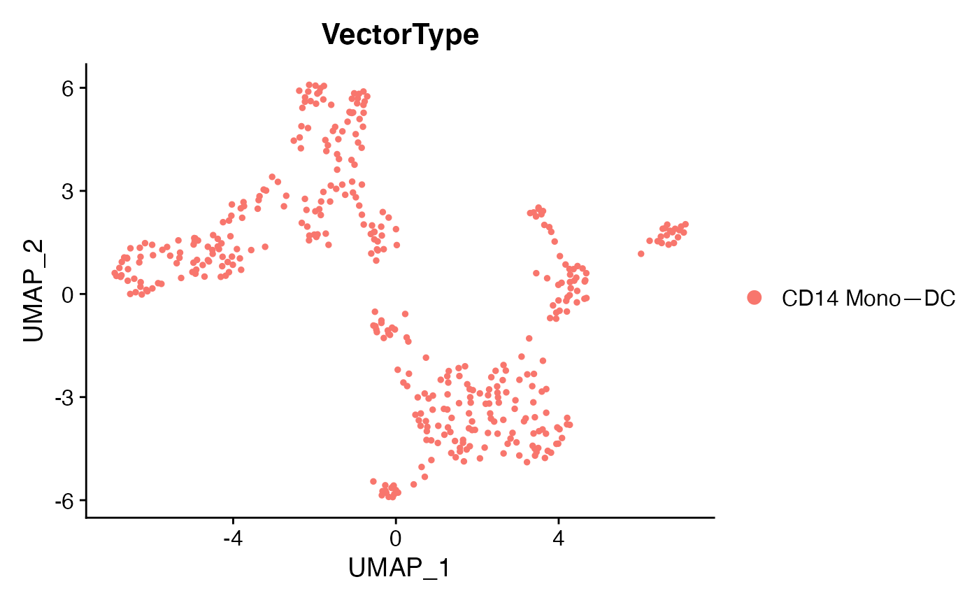
DimPlot(voi.data,group.by = 'Condition')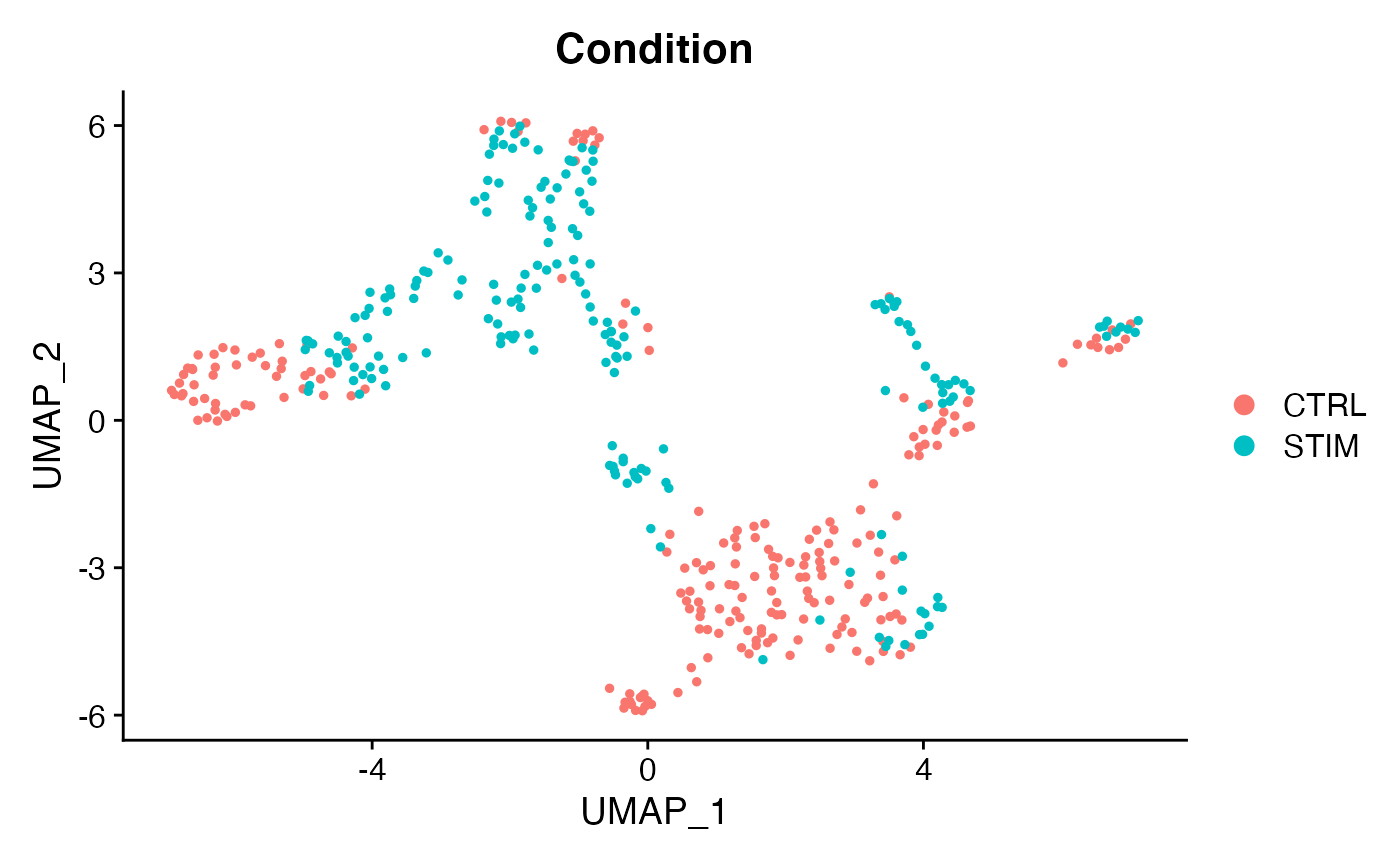
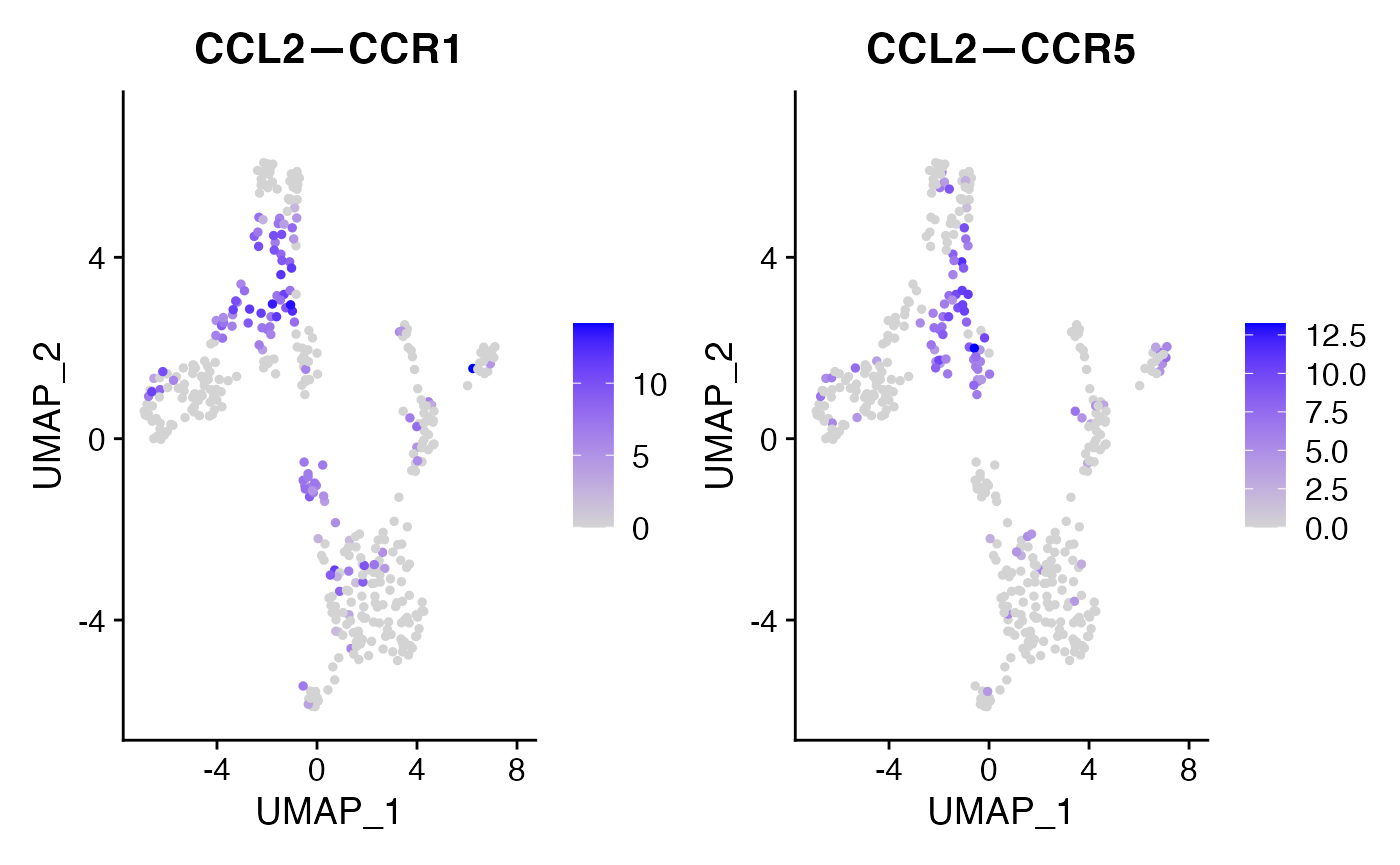
And we can then check that the markers we found earlier appear accurate:
FeaturePlot(voi.data,
            features = c('CCL2—CCR1','CCL2—CCR5'),max.cutoff = 150)