Pseudotemporal Ordering with NICHES
Micha Sam Brickman Raredon & Neeharika Kothapalli
2022-07-20
06 Pseudotime.RmdNICHES data can be overlaid onto pseudotemporal orderings. However, the exact way in which this is done matters a great deal for biologically interpretability. This vignette demonstrates one of the simplest and most manageable use-cases: asking how sensed microenvironment ‘changes’ with differentiation in a single homeostatic tissue. The ligand milieu in this case is constant (since we are dealing with a single system and the tissue itself has constant composition) but the receptor profile of a differentiating lineage will change over pseudotime. NICHES allows rapid observation of this changing interaction.
We leverage data from https://www.science.org/doi/10.1126/sciadv.aaw3851 to show this specific application.
Load Dependencies
require(Seurat)
require(NICHES)
require(monocle3)
library(dplyr)
library(ggplot2)
library(cowplot)
library(ComplexHeatmap)
library(SeuratWrappers)
library(Matrix)
library(patchwork)
library(magick)
set.seed(2)
We look at the whole dataset as a starting point (10,953 cells):
Load Data
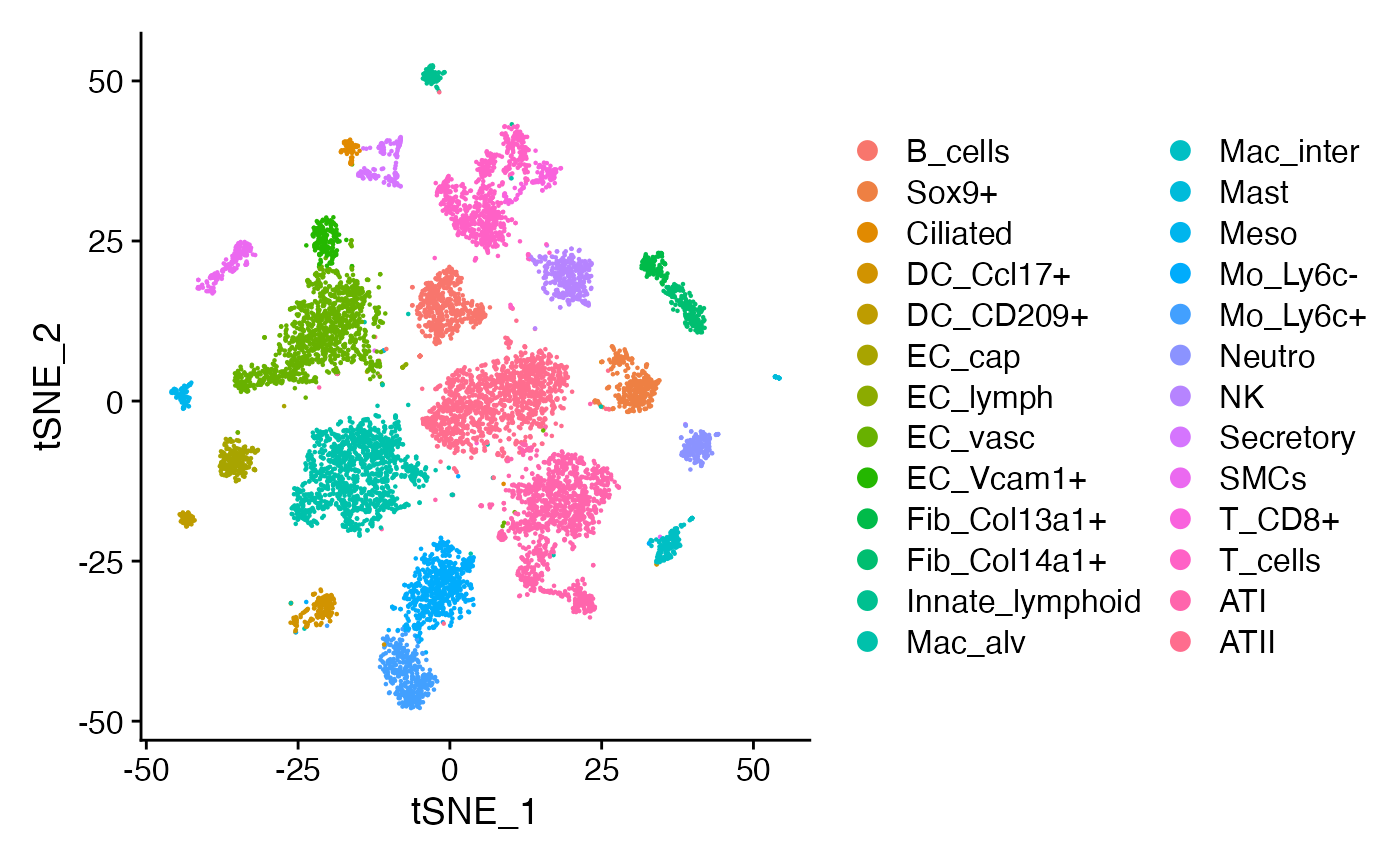
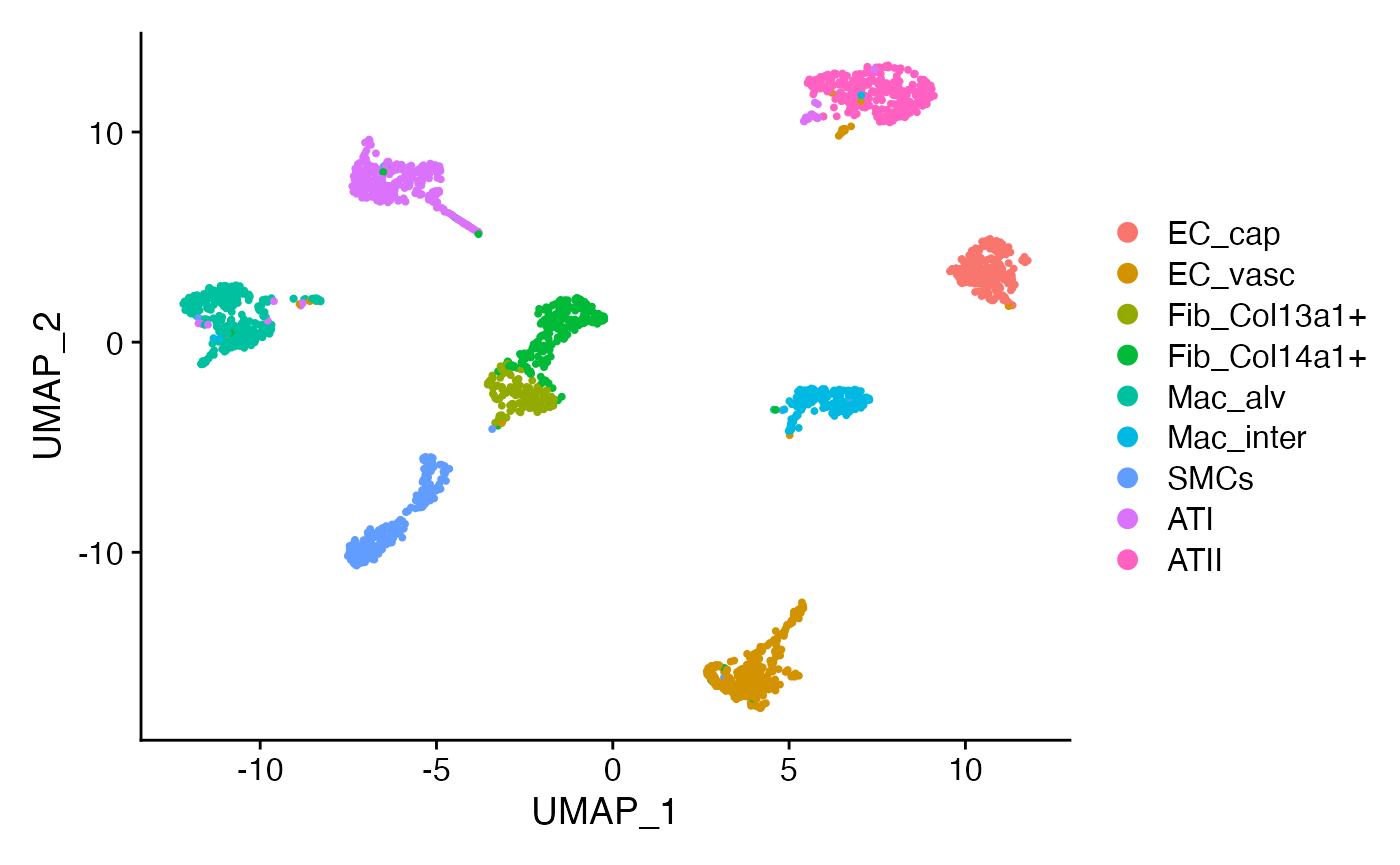
We are going to focus specifically on ATII-ATI epithelial differentiation. We want to ask what changes occur in the sensed microenvironment as ATII cells differentiate into ATI cells. For simplicity, we are going to again limit our analysis to 9 cell types that we are confident are often found in close proximity to both ATII and ATI cells in the alveolus of the lung:
Focus on histologically co-localized cell-system, and downsample for this vignette
rat.sub <- subset(rat,idents = c('ATII','ATI',
                                 'Mac_alv','Mac_inter',
                                 'Fib_Col13a1+','Fib_Col14a1+','SMCs',
                                 'EC_cap','EC_vasc'))
rat.sub <- subset(rat.sub,cells = WhichCells(rat.sub,downsample = 300))
rat.sub <- ScaleData(rat.sub)
rat.sub <- FindVariableFeatures(rat.sub)
rat.sub <- RunPCA(rat.sub)
ElbowPlot(rat.sub,ndims=50)
We then compute SystemToCell information within this cell-system and isolate the outputs corresponding to our two transdifferentiating cell types, as follows:
Visualization of homeostatic microenvironment for two transdifferentiating cell types
rat.sub@meta.data$cell_types <- Idents(rat.sub)

lung.niche <- RunNICHES(rat.sub,
                        assay = 'alra',
                        species = 'rat',
                        LR.database = 'fantom5',
                        cell_types = "cell_types",
                        SystemToCell = T,
                        CellToCell = F)
# Here we use a previously-created imputed data slot. The same computation may be performed on any data slot including standard log-normalized RNA values.
niche.object <- lung.niche$SystemToCell #Extract the output of interest

# Subset to receiving cells of interest
Idents(niche.object) <- niche.object@meta.data$ReceivingType
niche.object <- subset(niche.object,idents = c('ATII','ATI'))
niche.object <- ScaleData(niche.object) #Scale
niche.object <- FindVariableFeatures(niche.object,selection.method="disp") #Identify variable features
niche.object <- RunPCA(niche.object,npcs = 50) #RunPCA
ElbowPlot(niche.object,ndims=50) #Choose PCs to use for embedding
niche.object <- RunUMAP(niche.object,dims = 1:12) #Embed
DimPlot(niche.object,reduction = 'umap',label = T,repel = F,label.size = 6)+
  NoLegend()+ NoAxes()+ ggtitle('Alveolar Epithelial Microenvironment')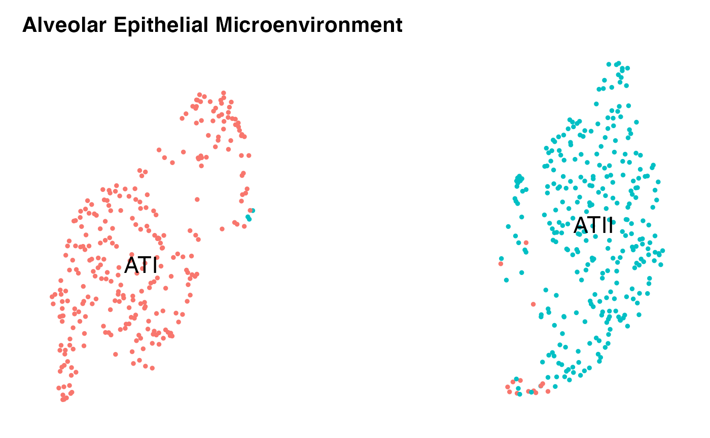
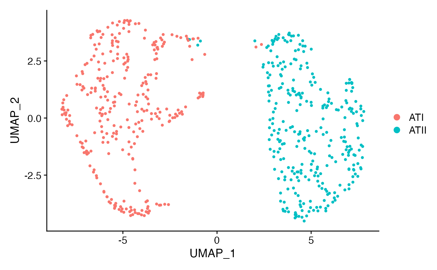
This is a good start and tells us we are on the right track. We can that some SystemToCell measurements classified as landing on an ATII are actually quantitatively similar to those landing on ATI cells. We can explore this in greater depth by pausing the analysis of the NICHES data, and taking the time to pseudotemporally order the original cells. Here, we use monocle3 to do this:
Pseudotemporal ordering of original cells
# Subset, run UMAP, take a look to check
cell.data <- subset(rat.sub,idents = c('ATII','ATI'))
cell.data <- ScaleData(cell.data)
cell.data <- FindVariableFeatures(cell.data)
cell.data <- RunPCA(cell.data)
ElbowPlot(cell.data,ndims=20)
# Convert to Monocle CDS
cell.cds <- as.cell_data_set(cell.data)
# Calculate size factors using built-in function in monocle3
#cell.cds <- estimate_size_factors(cell.cds)

# Make pseudotime trajectory with a known start point
cell.cds <- cluster_cells(cds = cell.cds, reduction_method = "UMAP")
cell.cds <- learn_graph(cell.cds, use_partition = F)
#>
  |
  |                                                                      |   0%
  |
  |======================================================================| 100%
start <- WhichCells(cell.data,idents = 'ATII')
cell.cds <- order_cells(cell.cds, reduction_method = "UMAP", root_cells = start)

# Plot pseudotime trajectory
plot_cells(
  cds = cell.cds,
  color_cells_by = "pseudotime",
  show_trajectory_graph = TRUE,
  cell_size = 0.5)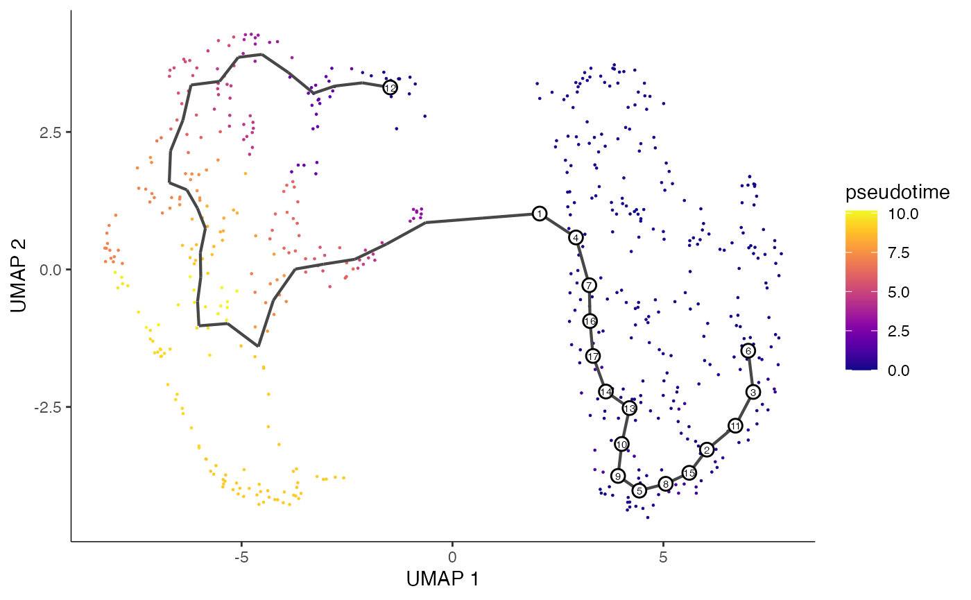
We can then map this pseudotemporal ordering back to the original Seurat object:
cell.data <- AddMetaData(
  object = cell.data,
  metadata = cell.cds@principal_graph_aux@listData$UMAP$pseudotime,
  col.name = "Pseudotime"
)

FeaturePlot(cell.data, c("Pseudotime"), pt.size = 0.4) & scale_color_viridis_c()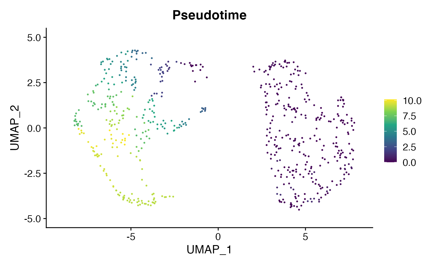
OR, we can map the pseudotemporal ordering on the NICHES SystemToCell object.
niche.object <- AddMetaData(
  object = niche.object,
  metadata = cell.cds@principal_graph_aux@listData$UMAP$pseudotime,
  col.name = "Pseudotime"
)

FeaturePlot(niche.object, c("Pseudotime"), pt.size = 0.4) & scale_color_viridis_c()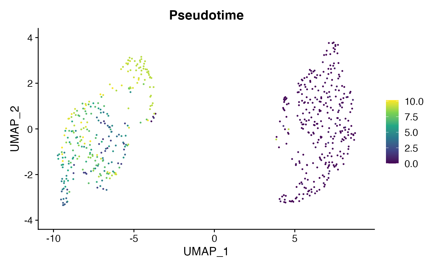
But more fundamentally, we are now set to see how signaling ‘changes’ over pseudotime, which was our original goal. Here is one approach for how to do this:
# Convert NICHES object to matrix format
data <-  as.matrix(niche.object@assays[["SystemToCell"]]@data)

# Count the percent of non-zeros for each mechanism
temp <- apply(data,1,function(z){
  n <- 1-sum(z==0)/dim(data)[2]
})
temp <- temp[which(temp>0.25)] # Remove mechanisms with more than 75% of zeros
mechs <- names(temp)
data <- data[mechs,] # 836 mechs

# Pull metadata
meta <- niche.object@meta.data
meta$cell <- rownames(meta)

# Run Pearson correlation for each mechanism against pseudotime
df <- data.frame()
for(i in 1:length(mechs)){
  temp <- data.frame(data = data[i,])
  colnames(temp) <- "data"
  temp$cell <- rownames(temp)
  temp <- merge(temp,meta,by="cell")
  test <- cor.test(temp$Pseudotime,temp$data)
  row = data.frame(mech = rownames(data)[i],p.val = test[["p.value"]], cor = test[["estimate"]][["cor"]])
  df <- rbind(df,row)
}

# Subset to mechanisms with desired thresholds
df$q.val= p.adjust(df$p.val, method = "fdr")
plot <- df[which(df$q.val<0.05),]
plot <- plot[which(plot$mech %in% mechs),]
plot <- plot[which(abs(plot$cor)>.8),] # Looking for high correlations with pseudotime
to_plot <- as.matrix(data[plot$mech,])

# Arrange metadata and cells by pseudotime
meta <- meta %>% arrange(Pseudotime)
to_plot <- to_plot[,meta$cell]

# Prepare Annotations
ha <- HeatmapAnnotation(df = meta[,c('Pseudotime','ReceivingType')],which = 'column')

# Scale for visualization
to_plot_scale <- t(scale(t(to_plot), center = TRUE, scale = TRUE)) # scale data for better visualization

# Plot in HeatMap Form
Heatmap(to_plot_scale,
        column_order = meta$cell,
        show_column_names = FALSE,
        show_row_names = TRUE,
        top_annotation = ha,
        use_raster = T)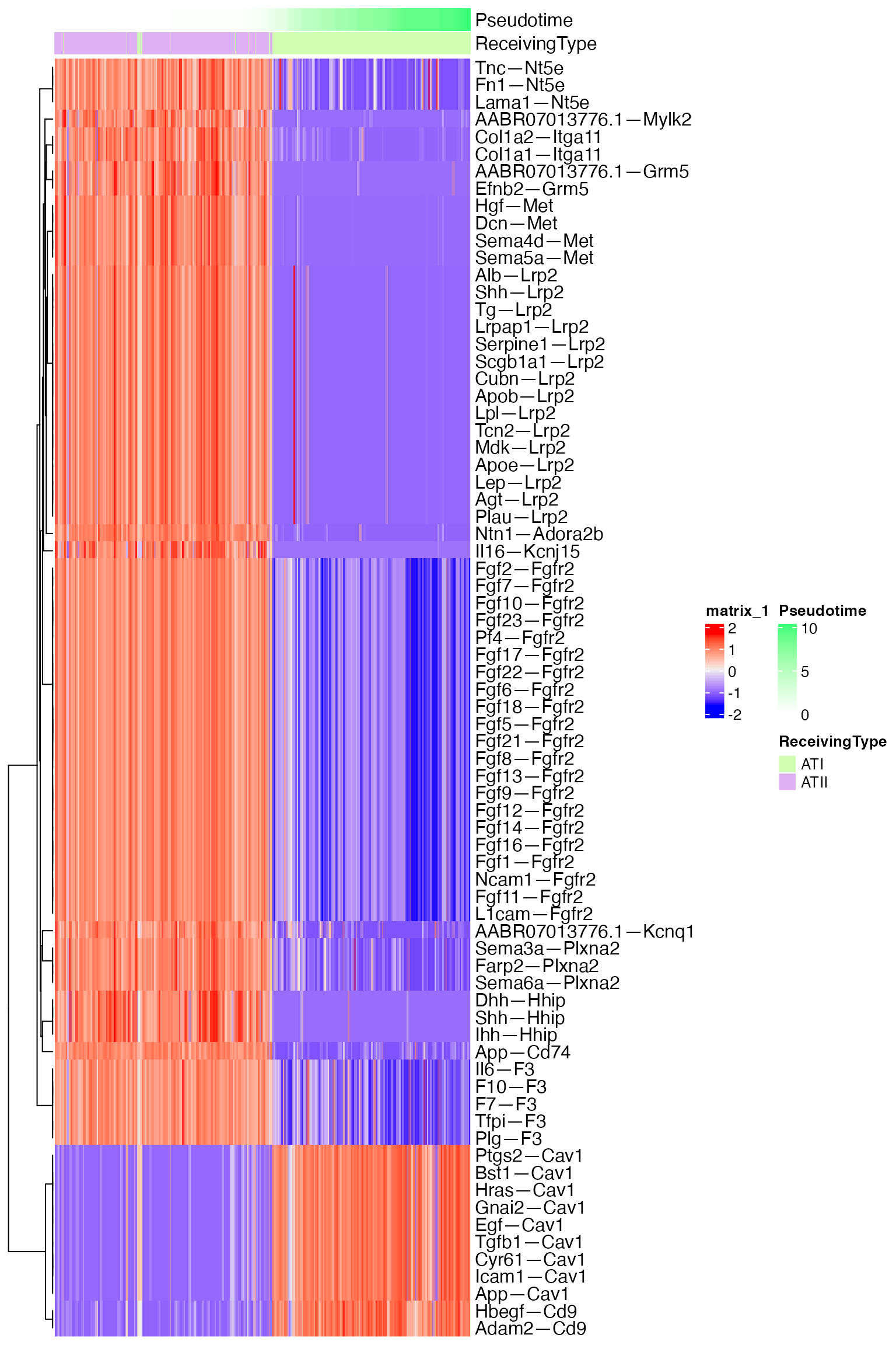
The altered sensed-signaling through Fgfr2, Hhip, and Met are all particularly biologically relevant in this instance.
These observed patterns are only dependent on receptor expression, and therefore could have been found through traditional transcriptomic analysis. Because NICHES operates on a mechanism level, however, this approach narrows focus exclusively onto receptors which have cognate ligand being expressed within the system.
It should be noted that NICHES is also a powerful tool for pseudotemporal investigation of processes in which both the ligand milieu and the receptor expression of a differentiating lineage are changing. This will be covered in a separate vignette, since it is a distinct biologic application and is more complicated to implement.