System Effects of Aberrant Cells

In this vignette we show how the SystemToCell functionality of NICHES can be used to probe the hypothetical effects of aberrant additional cell populations in tissues. We leverage data from https://www.science.org/doi/10.1126/sciadv.aba1983 (10.1126/sciadv.aba1983) for this.

Load Dependencies

require(Seurat)
require(SeuratWrappers)
require(NICHES)
library(ggplot2)
library(cowplot)
library(dplyr)

Here, we use data from 10.1126/sciadv.aba1983, downsampled for this demonstration and saved publicly on Zenodo:

Load Data

# # Load data and assemble objects
# setwd("/Volumes/Samsung_T5/Kaminski_Lab")
# expression_matrix <- Matrix::readMM('GSE136831_RawCounts_Sparse.mtx.gz')
# features <- read.table('GSE136831_AllCells.GeneIDs.txt.gz',header = T)
# barcodes <- read.table('GSE136831_AllCells.cellBarcodes.txt.gz',header = F)
# meta_data <- read.table("/Volumes/Samsung_T5/Kaminski_Lab/GSE136831_AllCells.Samples.CellType.MetadataTable.txt.gz",header = T,row.names = 'CellBarcode_Identity')
# dimnames(expression_matrix) = list(features$HGNC_EnsemblAlt_GeneID,barcodes$V1)
# seurat_object <- CreateSeuratObject(counts = expression_matrix)
# seurat_object <- AddMetaData(seurat_object,metadata = meta_data)
# table(seurat_object$Disease_Identity)
# Idents(seurat_object) <- seurat_object$Disease_Identity
# ipf <- subset(seurat_object,idents = 'IPF')
# Idents(ipf) <- ipf$Manuscript_Identity
# control <- subset(seurat_object,idents = 'Control')
# Idents(control) <- control$Manuscript_Identity
# 
# # Downsample for vignette
# table(Idents(ipf))
# ipf.down <- subset(ipf,cells = WhichCells(ipf,downsample = 3000))
# table(Idents(ipf.down))
# table(Idents(control))
# control.down <- subset(control,cells = WhichCells(control,downsample = 3000))
# table(Idents(control.down))
# 
# # Save for reference
# save(ipf.down,file='ipf.down.Robj')
# save(control.down,file='control.down.Robj')
# 
# # Clean up
# rm(barcodes)
# rm(features)
# rm(meta_data)
# rm(expression_matrix)
# rm(seurat_object)
# gc()

# Load from save
load('ipf.down.Robj')
load('control.down.Robj')

For demonstration, let’s limit our analysis to celltypes that we know co-localize near each other in lung tissue. Note that the aberrant basaloid cells are only present in IPF tissue and not in control tissue. We standardize the total cell number in each condition so that the mean operator used to quantify the total ligand production within each system uses the same denominator.

Subset and standardize cell number


COI <- c('ATII','ATI','Aberrant_Basaloid',
         'Macrophage_Alveolar',
         'VE_Capillary_A','VE_Capillary_B',
         'Fibroblast')
ipf.sub <- subset(ipf.down,idents = COI)
control.sub <- subset(control.down,idents = COI[!(COI == 'Aberrant_Basaloid')])

# Downsample to make each system the same size
Idents(ipf.sub) <- ipf.sub@meta.data$Disease_Identity
Idents(control.sub) <- control.sub@meta.data$Disease_Identity

num <- min(ncol(ipf.sub),ncol(control.sub))

ipf.sub <- subset(ipf.sub,cells = WhichCells(ipf.sub,downsample = num))
control.sub <- subset(control.sub,cells = WhichCells(control.sub,downsample = num))

# Set cell labels as identity
Idents(ipf.sub) <- ipf.sub$Manuscript_Identity
Idents(control.sub) <- control.sub$Manuscript_Identity

# Observe different celltype distributions
distribution.1 <- data.frame(table(Idents(ipf.sub)))
distribution.1$Condition <- 'IPF'
distribution.2 <- data.frame(table(Idents(control.sub)))
distribution.2$Condition <- 'CTRL'
distribution <- rbind(distribution.1,distribution.2)
ggplot(data = distribution,
       aes(x = Var1,y=Freq,fill = Condition))+
  geom_bar(stat='identity',position='dodge')+
  theme(axis.text.x = element_text(angle = 45, vjust = 1, hjust=1))+
  ggtitle('Number of Cells Per Condition')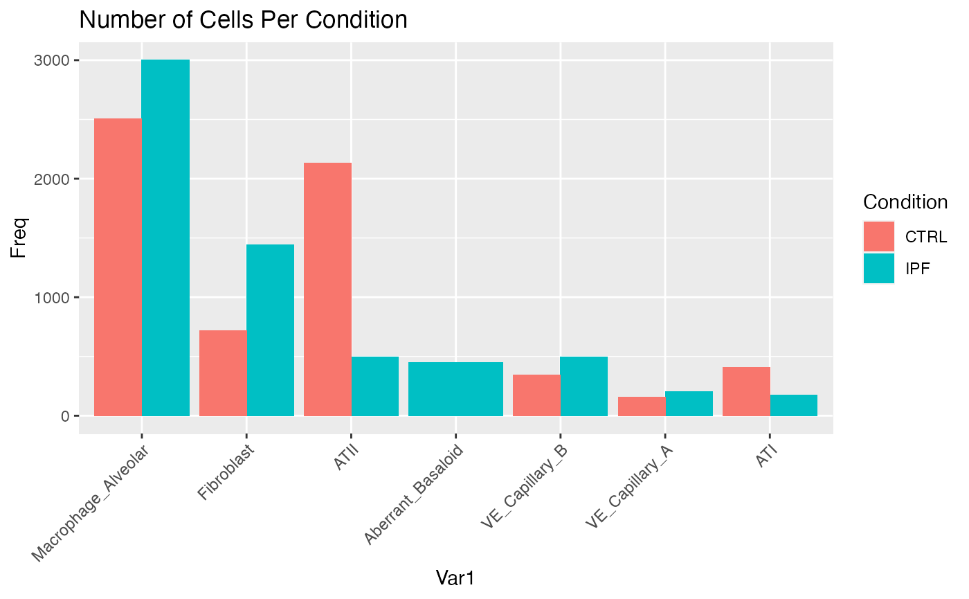


# Double check that systems are the same size
ncol(ipf.sub) == ncol(control.sub)
#> [1] TRUE

Define the question being investigated

We want to know how the presence of disease-specific Aberrant Basaloid cells in IPF affect the sensed signaling milieu of other cells. In other words, we are asking:

How does the cell-signaling milieu in IPF tissue differ from that in control tissue, given that there is an additional cell population in the IPF disease tissue?

We approach this as follows:

Run SystemToCell for each system individually

# Run NICHES on each system and store/name the outputs
data.list <- list(ipf.sub,control.sub)
names(data.list) <- c('IPF','CTRL')
scc.list <- list()
for(i in 1:length(data.list)){
  print(i)
  data.list[[i]] <- NormalizeData(data.list[[i]])
  scc.list[[i]] <- RunNICHES(data.list[[i]],
                             LR.database="fantom5",
                             species="human",
                             assay="RNA",
                             cell_types = 'stash',
                             min.cells.per.ident=1,
                             min.cells.per.gene = 50,
                             meta.data.to.map = c('Disease_Identity','Manuscript_Identity'),
                             SystemToCell = T,
                             CellToCell = F,
                             blend = 'mean')
}
#> [1] 1
#> [1] 2
names(scc.list) <- names(data.list)

Isolate NICHES output of interest

temp.list <- list()
for(i in 1:length(scc.list)){
temp.list[[i]] <- scc.list[[i]]$SystemToCell # Isolate SystemToCell Signaling, which is all that will be covered in this vignette
temp.list[[i]]$Condition <- names(scc.list)[i] # Tag with metadata
}

Merge the NICHES output information and check data quality

# Merge together
scc.merge <- merge(temp.list[[1]],temp.list[2])

# Clean up low-information crosses
VlnPlot(scc.merge,features = 'nFeature_SystemToCell',group.by = 'Condition',pt.size=0.1,log = T)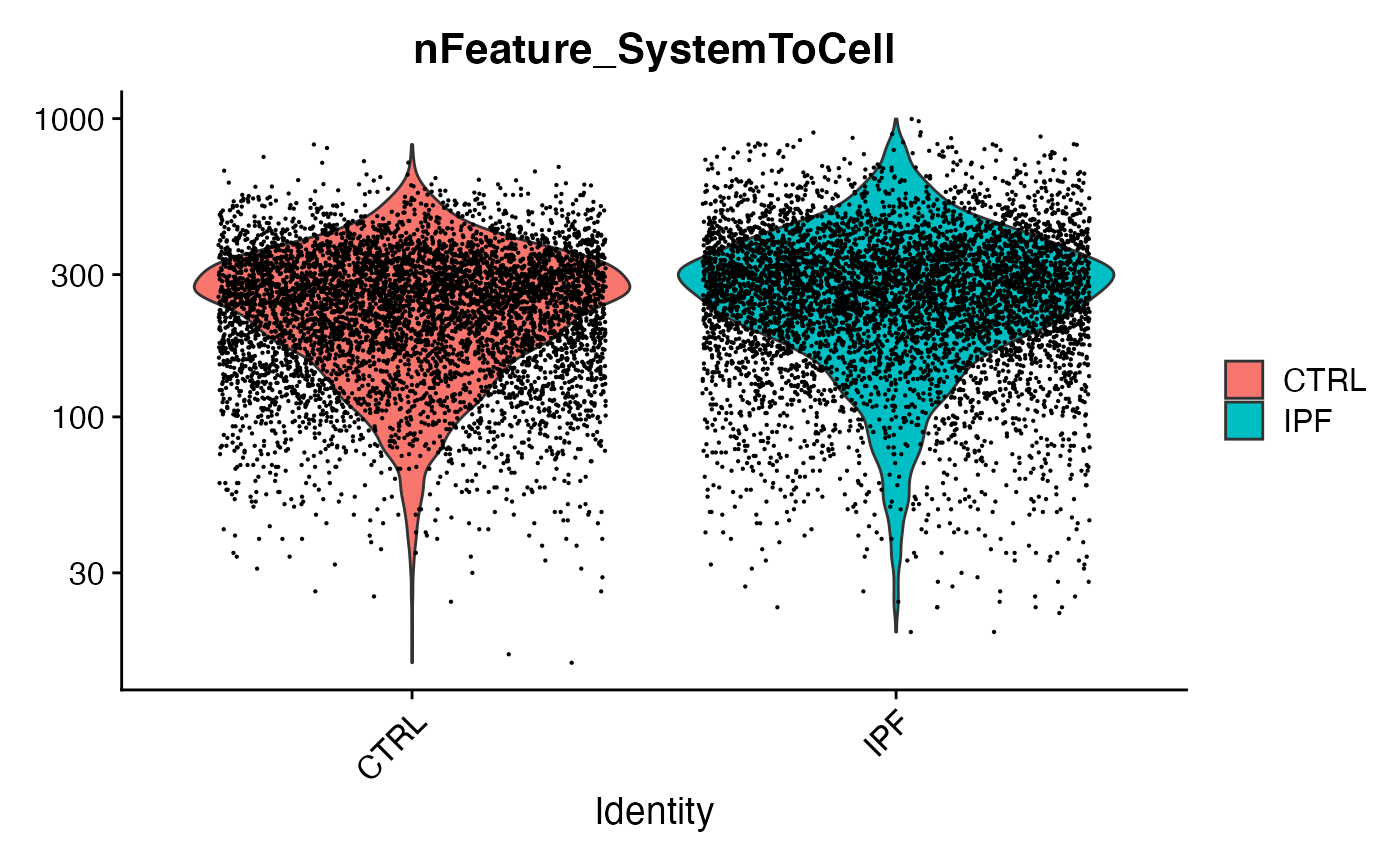

scc.sub <- subset(scc.merge,nFeature_SystemToCell > 5) # Requesting at least 5 distinct ligand-receptor interactions per measurement

Let’s now perform an initial visualization of SystemToCell signaling between these two conditions:

Visualize the dataset, comparing SystemToCell signaling between IPF and Control tissue

# Perform initial visualization
scc.sub <- ScaleData(scc.sub)
scc.sub <- FindVariableFeatures(scc.sub)
scc.sub <- RunPCA(scc.sub,npcs = 100)
ElbowPlot(scc.sub,ndim=100)

We choose to use the first 25 principle components for a first embedding:

scc.sub <- RunUMAP(scc.sub,dims = 1:25)
p1 <- DimPlot(scc.sub,group.by = 'Condition')
p2 <- DimPlot(scc.sub,group.by = 'ReceivingType')
plot_grid(p1,p2)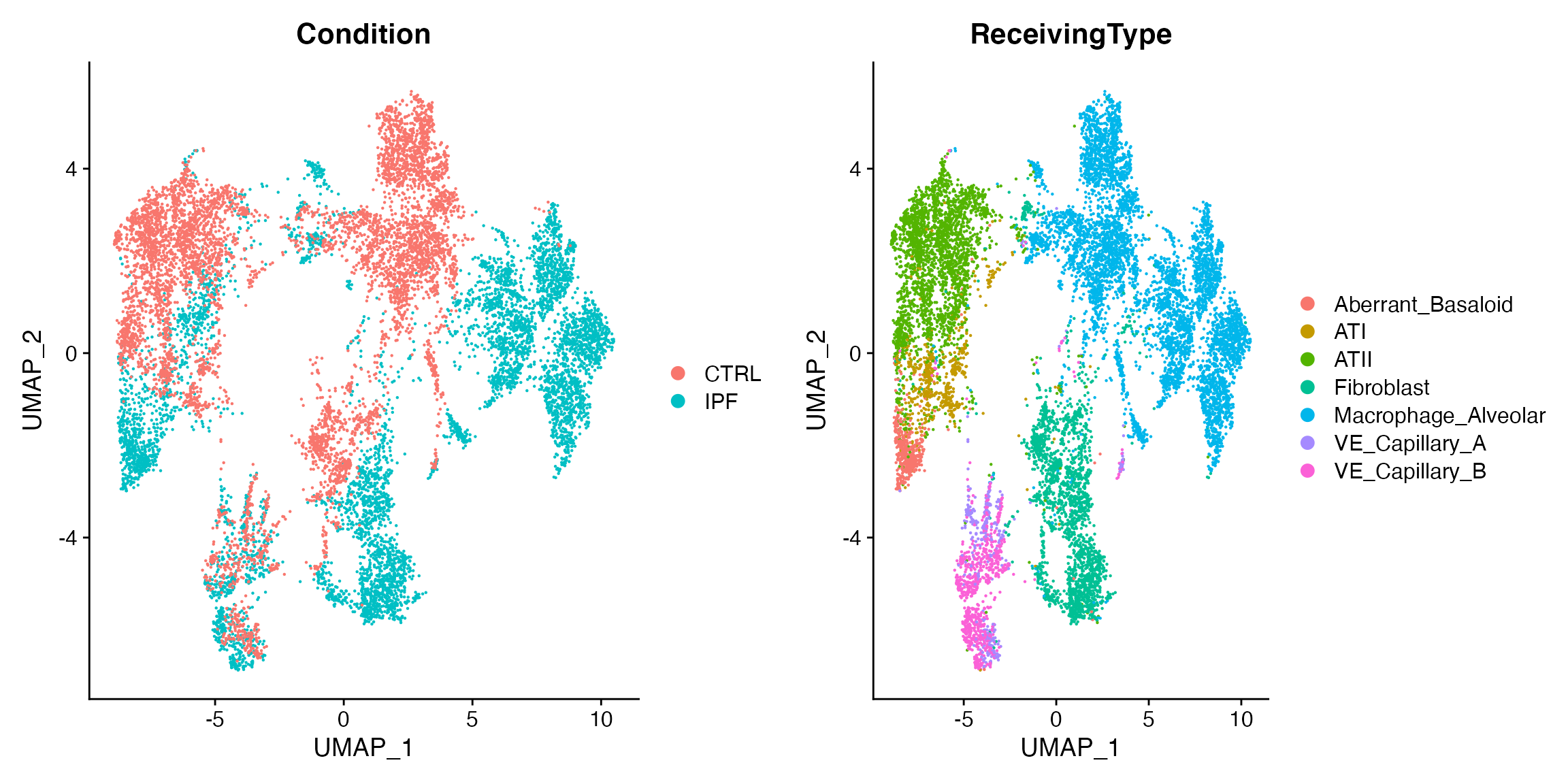

This presents us with some very interesting opportunities for analysis. IPF is a disease in which fibroblasts and macrophages are signficantly disregulated, and we can see here that their signaling milieus are perturbed in IPF as compared to control. (In contrast, the capillary endothelial cells do not appear to have a greatly-perturbed milieu when considering this very limited demonstration cell-system.) We can probe the altered fibroblast milieu more fully as follows:

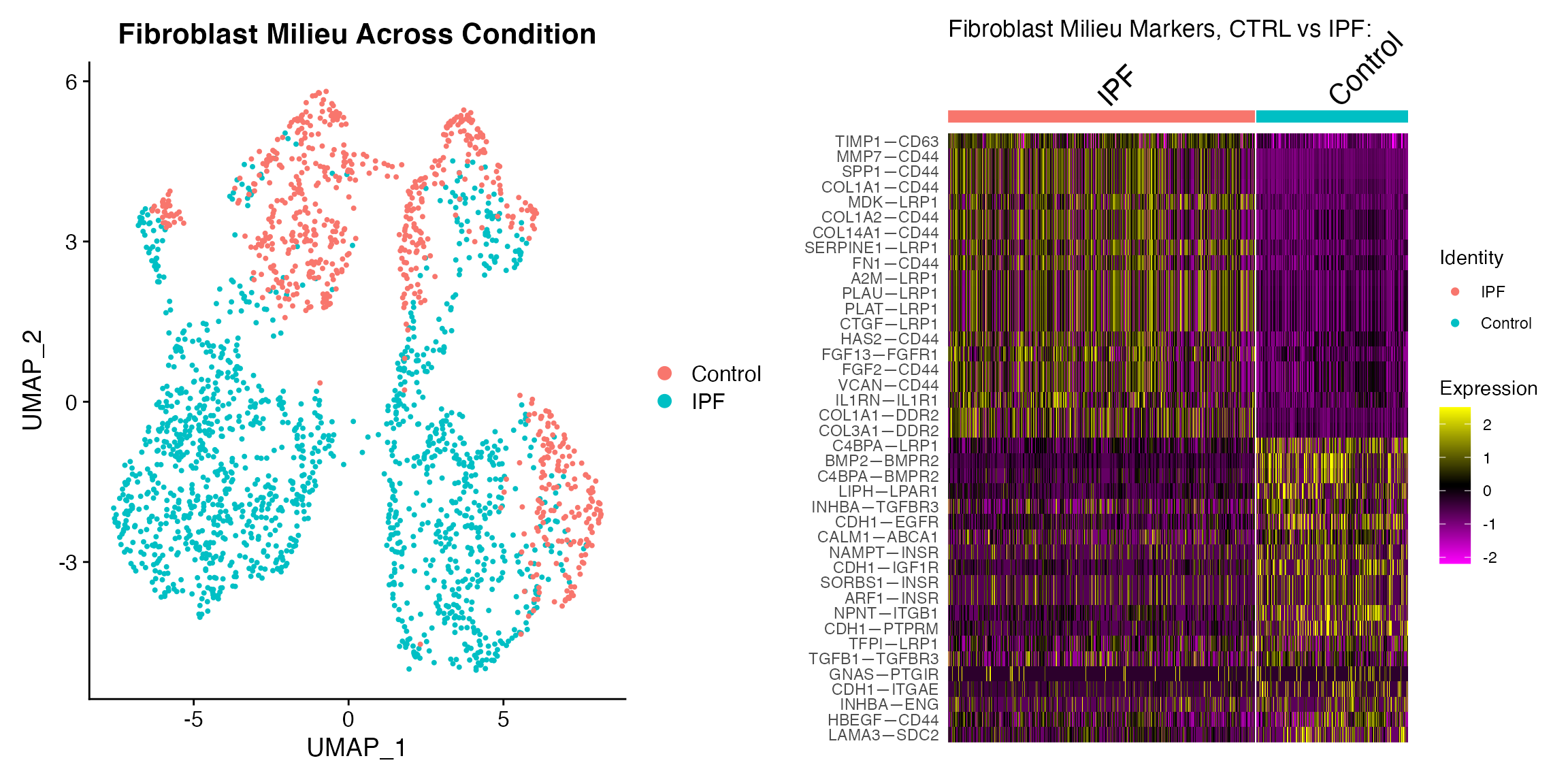
Examine Fibroblast Milieu Across Condition

COI <- 'Fibroblast'
subs <- subset(scc.sub, idents = COI)
subs <- ScaleData(subs)
subs <- RunPCA(subs)
subs <- RunUMAP(subs,dims = 1:5)
p1 <- DimPlot(subs,group.by = 'Disease_Identity')+ ggtitle('Fibroblast Milieu Across Condition')

# Find markers (here we use ROC)
Idents(subs) <- subs$Disease_Identity
markers <- FindAllMarkers(subs, test.use = "roc",assay='SystemToCell',
                          min.pct = 0.1,logfc.threshold = 0.1,
                          return.thresh = 0.1,only.pos = T)

# Subset to top 20 markers per condition
top20 <- markers %>% group_by(cluster) %>% top_n(n = 20, wt = myAUC)

# Make a heatmap
p2 <- DoHeatmap(subs,group.by="ident",features=top20$gene, assay="SystemToCell") +  
  ggtitle("Fibroblast Milieu Markers, CTRL vs IPF: ")

plot_grid(p1,p2)

Micha Sam Brickman Raredon & Neeharika Kothapalli

2022-07-20