Converting Single-Cell Atlases to Single-Cell Signaling Atlases

Micha Sam Brickman Raredon & Junchen Yang

2022-07-20

NICHES is able to rapidly convert traditional single-cell atlases into single-cell signaling atlases which allow cell-cell signaling to be analyzed using existing single-cell software. Here, we leverage publicly available PBMC data to demonstrate:

Load Dependencies

library(Seurat)
library(SeuratData)
library(SeuratWrappers)
library(NICHES)
library(dplyr)
library(ggplot2)

Load and Visualize Single-Cell Data

Here, we use the ‘pbmc3k’ dataset from SeuratData. This is a commonly-used dataset showing options for the workflow.

InstallData("pbmc3k")
data("pbmc3k")
Idents(pbmc3k) <- pbmc3k$seurat_annotations
pbmc3k <- ScaleData(pbmc3k)
pbmc3k <- FindVariableFeatures(pbmc3k)
pbmc3k <- RunPCA(pbmc3k)
ElbowPlot(pbmc3k,ndims=50)

pbmc3k <- RunUMAP(pbmc3k,dims = 1:10)
DimPlot(pbmc3k,reduction = 'umap',label = T,repel = F,label.size = 6)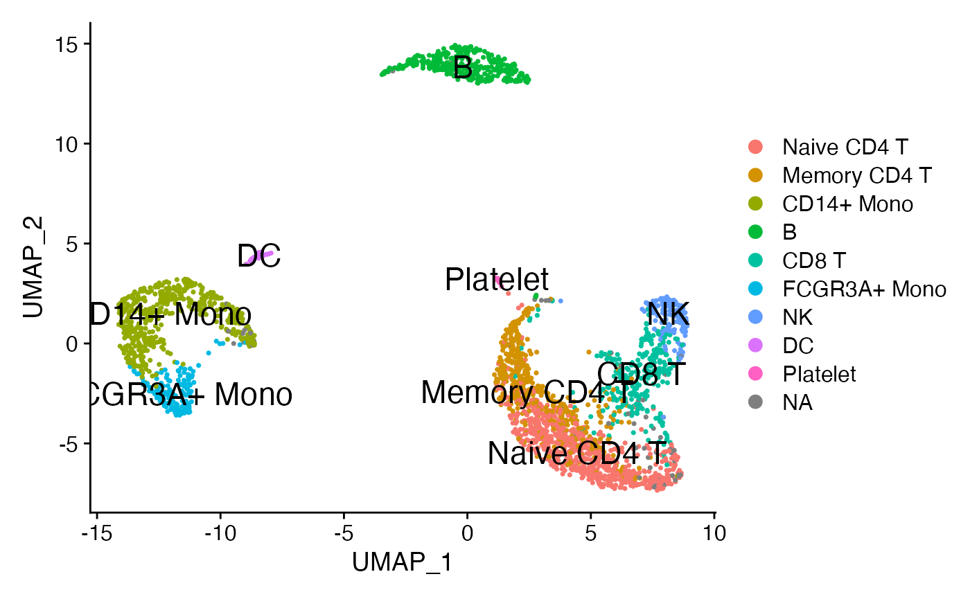

For simplicity, let’s focus in on signaling within a simple 3-cell system:

sub <- subset(pbmc3k,idents = c('B','Naive CD4 T','CD14+ Mono'))
DimPlot(sub,reduction = 'umap',label = T,repel = F,label.size = 6)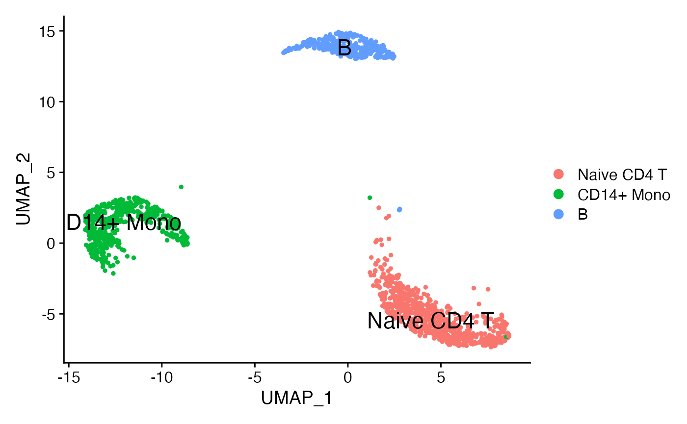

Convert to Cell-Cell Signaling Atlas

Here, we use the human-specific OmniPath database as our ground-truth ligand-receptor mechanism database, which includes some mechanisms with more than one subunit on both the sending and receiving arms:

scc <- RunNICHES(sub,
                 assay = 'RNA',
                 species = 'human',
                 LR.database = 'omnipath',
                 cell_types = 'seurat_annotations',
                 CellToCell = T)

Visualize Cell-Cell Signaling Relationships using UMAP

We can visualize cell-cell signaling relationships quickly using tSNE or UMAP as follows:

demo <- scc$CellToCell
demo <- ScaleData(demo)
demo <- RunPCA(demo,features = rownames(demo))
ElbowPlot(demo,ndims=50)

PCHeatmap(demo,dims = 1:6,balanced = T,cells = 100)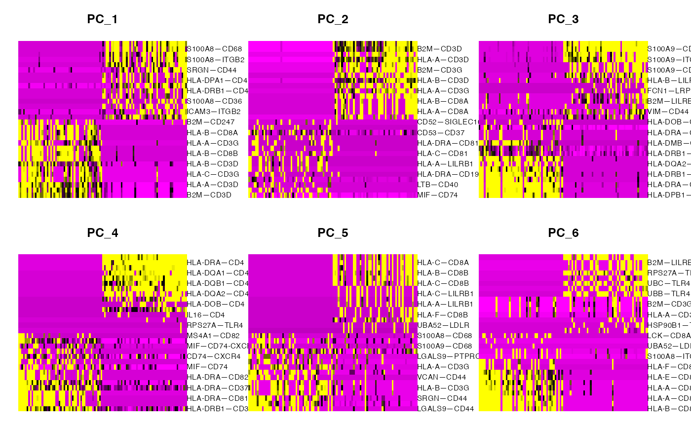

demo <- RunUMAP(demo,dims = 1:6)
DimPlot(demo,reduction = 'umap',group.by = 'VectorType',label = F)

This allows us to see some patterns and segregation of cell-cell relationships, however, this doesn’t look particularly clean. This is because the cell types that we have chosen here overlap significantly in the mechanisms that they employ. If we want to further clarify patterns that might not otherwise be obvious, we can run NICHES on the same data but imputed to amplify low-strength signal and remove gene-sampling-related clustering artifacts:

imputed <- SeuratWrappers::RunALRA(sub)
scc.imputed <- RunNICHES(imputed,
                 assay = 'alra',
                 species = 'human',
                 LR.database = 'omnipath',
                 cell_types = 'seurat_annotations',
                 CellToCell = T)
demo.2 <- scc.imputed$CellToCell
demo.2 <- ScaleData(demo.2)
demo.2 <- RunPCA(demo.2,features = rownames(demo.2))
ElbowPlot(demo.2,ndims=50)

PCHeatmap(demo.2,dims = 1:6,balanced = T,cells = 100)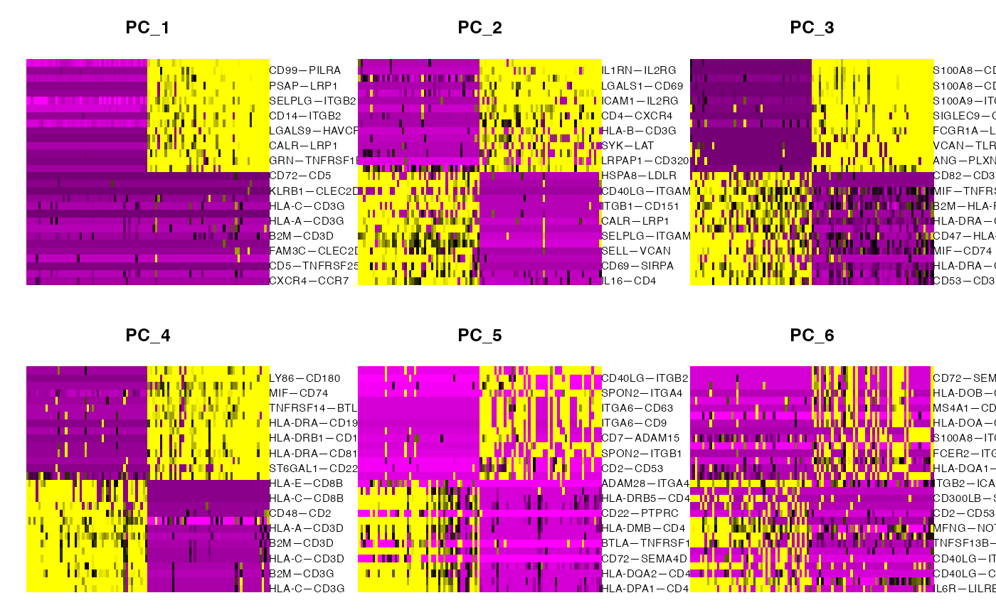

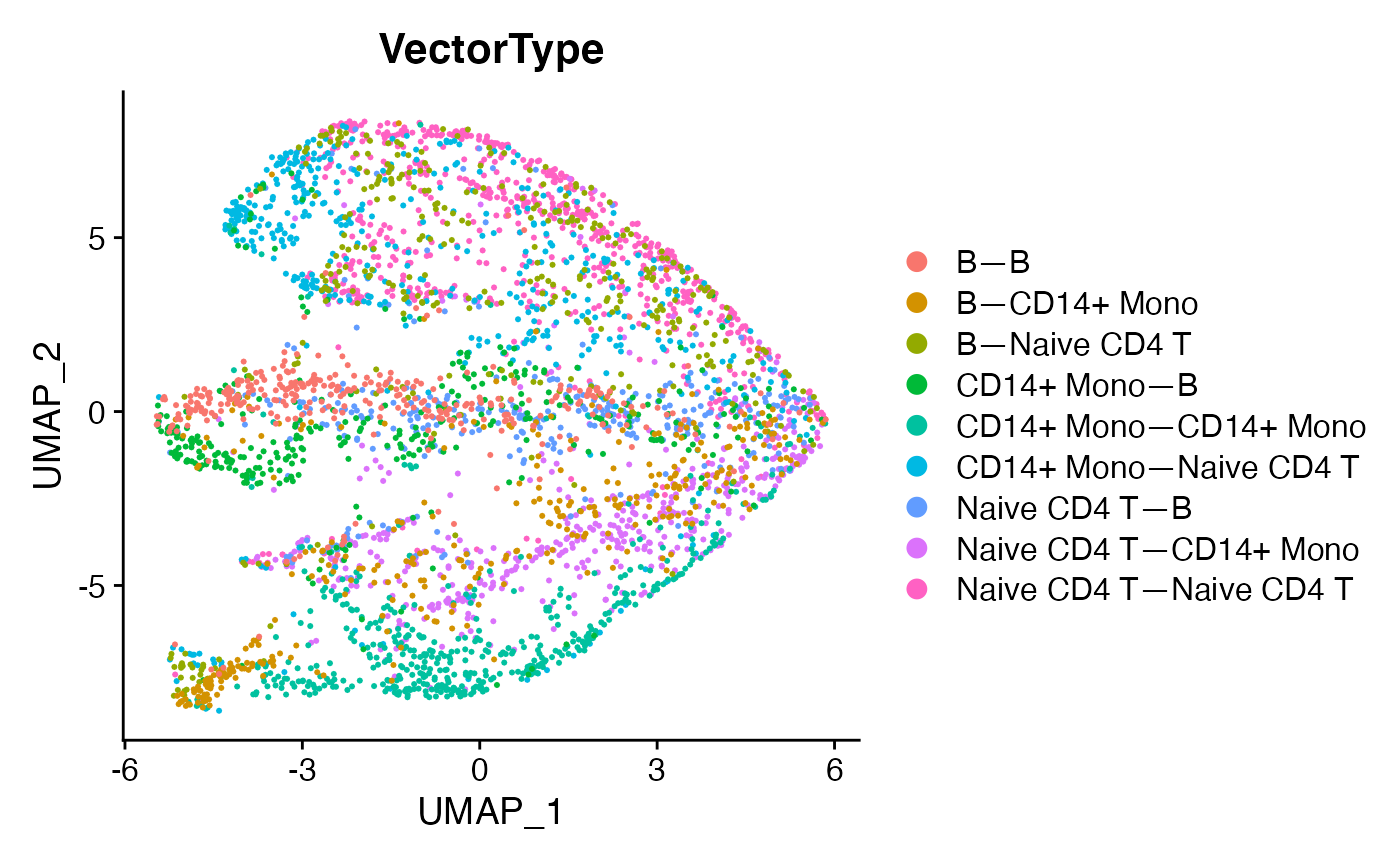
demo.2 <- RunUMAP(demo.2,dims = 1:6)
DimPlot(demo.2,reduction = 'umap',group.by = 'VectorType',label = F)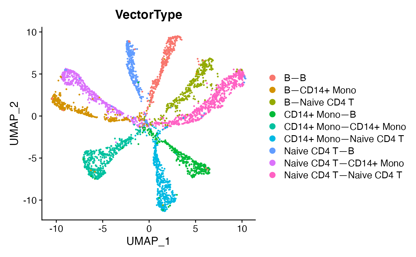

This looks cleaner, removes sampling-related artifacts, and allows clearer observation of relationships which occupy their own region of mechanism-space versus overlap with other cell-cell relationships. Differential expression can be run to identify prominent marker mechanisms as follows:

# Find markers
mark <- FindAllMarkers(demo.2,min.pct = 0.25,only.pos = T,test.use = "roc")
GOI_niche <- mark %>% group_by(cluster) %>% top_n(5,myAUC)
DoHeatmap(demo.2,features = unique(GOI_niche$gene))+ 
  scale_fill_gradientn(colors = c("grey","white", "blue"))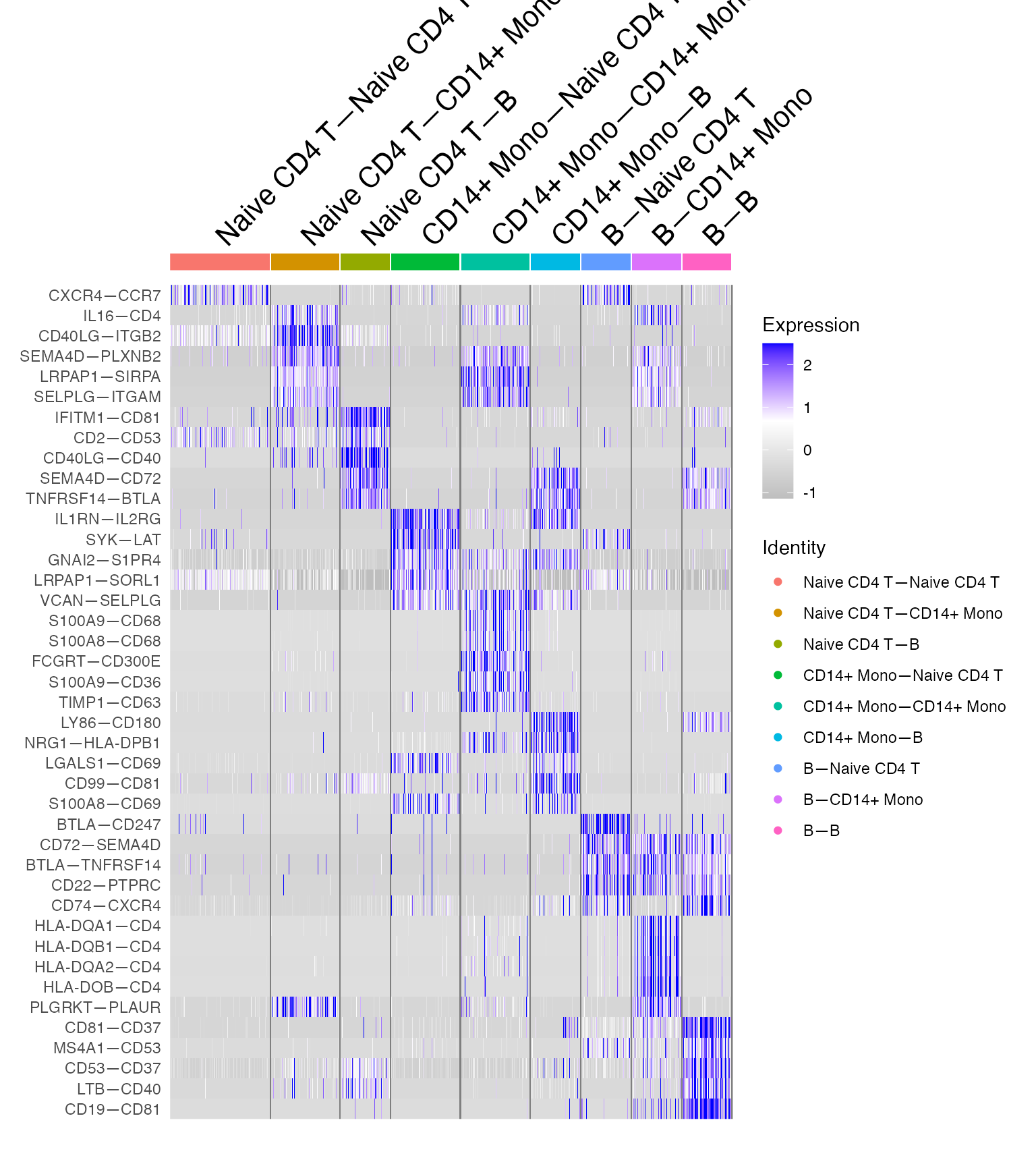

Which allows immediate recognition and confirmation of known biological truths such as CD40LG-CD40 preferentially mediating information transfer from T to B cells.