Cellular Relationships in the Rat Alveolus
Micha Sam Brickman Raredon & Junchen Yang
2022-07-20
03 Rat Alveolus.RmdIn this vignette we explore cellular microenvironment, cellular influence, and specific cell-cell relationships in the rat alveolus leveraging data from https://www.science.org/doi/10.1126/sciadv.aaw3851
Load Dependencies
require(Seurat)
require(SeuratWrappers)
require(ggpubr)
require(NICHES)
library(SeuratData)
library(Connectome)
library(ggplot2)
library(cowplot)
library(ComplexHeatmap)
library(ggthemes)
library(dplyr)
library(gridExtra)
library(igraph)
library(TSCAN)
library(ggbeeswarm)
library(writexl)
library(RColorBrewer)
First, let’s take a look at the whole dataset (10,953 cells), which has already been ALRA-imputed for this vignette and is publicly available on Zenodo:
Load Data
load("raredon_2019_rat.Robj")
#load(url('https://zenodo.org/record/6846618/files/raredon_2019_rat.Robj'))
TSNEPlot(rat)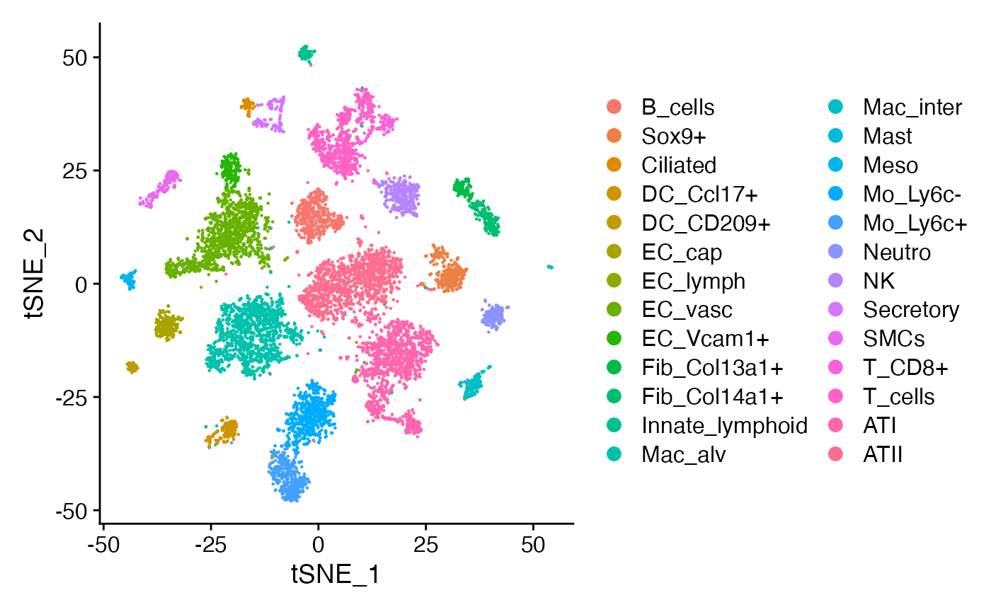
It is important to note that not all of these cell types are localized close together in the same region of tissue. Let’s limit our analysis to 9 celltypes that we are confident co-localize within the same region of tissue, namely, the alveolus:
rat.sub <- subset(rat,idents = c('ATII','ATI',
                                 'Mac_alv','Mac_inter',
                                 'Fib_Col13a1+','Fib_Col14a1+','SMCs',
                                 'EC_cap','EC_vasc'))
We may then compute and explore the character of different cellular ‘niches’ (System-to-Cell signaling networks) within this specific cell-system, as follows:
rat.sub@meta.data$cell_types <- Idents(rat.sub)

lung.niche <- RunNICHES(rat.sub,
                        assay = 'alra',
                        species = 'rat',
                        LR.database = 'fantom5',
                        cell_types = "cell_types",
                        SystemToCell = T,
                        CellToCell = F)
# Here we use a previously-created imputed data slot. The same computation may be performed on any data slot including standard log-normalized RNA values.
niche.object <- lung.niche$SystemToCell #Extract the output of interest
niche.object <- ScaleData(niche.object) #Scale
niche.object <- FindVariableFeatures(niche.object,selection.method="disp") #Identify variable features
niche.object <- RunPCA(niche.object,npcs = 100) #RunPCA
ElbowPlot(niche.object,ndims=100) #Choose PCs to use for embedding
niche.object <- RunUMAP(niche.object,dims = 1:15) #Embed
DimPlot(niche.object,reduction = 'umap',label = T,repel = F,label.size = 6)+
  NoLegend()+ NoAxes()+ ggtitle('Alveolar Microenvironment')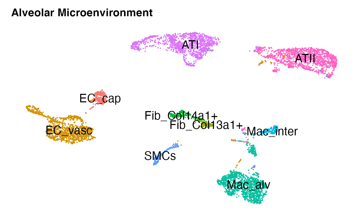
Each dot in the plot above represents an individual System-to-Cell network landing on a given receiving cell within this alveolar cell-system. We may identify markers for each celltype or cluster as follows:
#Markers
Idents(niche.object) <- niche.object[['ReceivingType']]
mark <- FindAllMarkers(niche.object,logfc.threshold = 1,min.pct = 0.5,only.pos = T,test.use = 'roc')

# Pull markers of interest to plot
mark$ratio <- mark$pct.1/mark$pct.2
marker.list <- mark %>% group_by(cluster) %>% top_n(5,avg_log2FC)

#Plot in Heatmap form
DoHeatmap(niche.object,features = marker.list$gene,cells = WhichCells(niche.object,downsample = 100))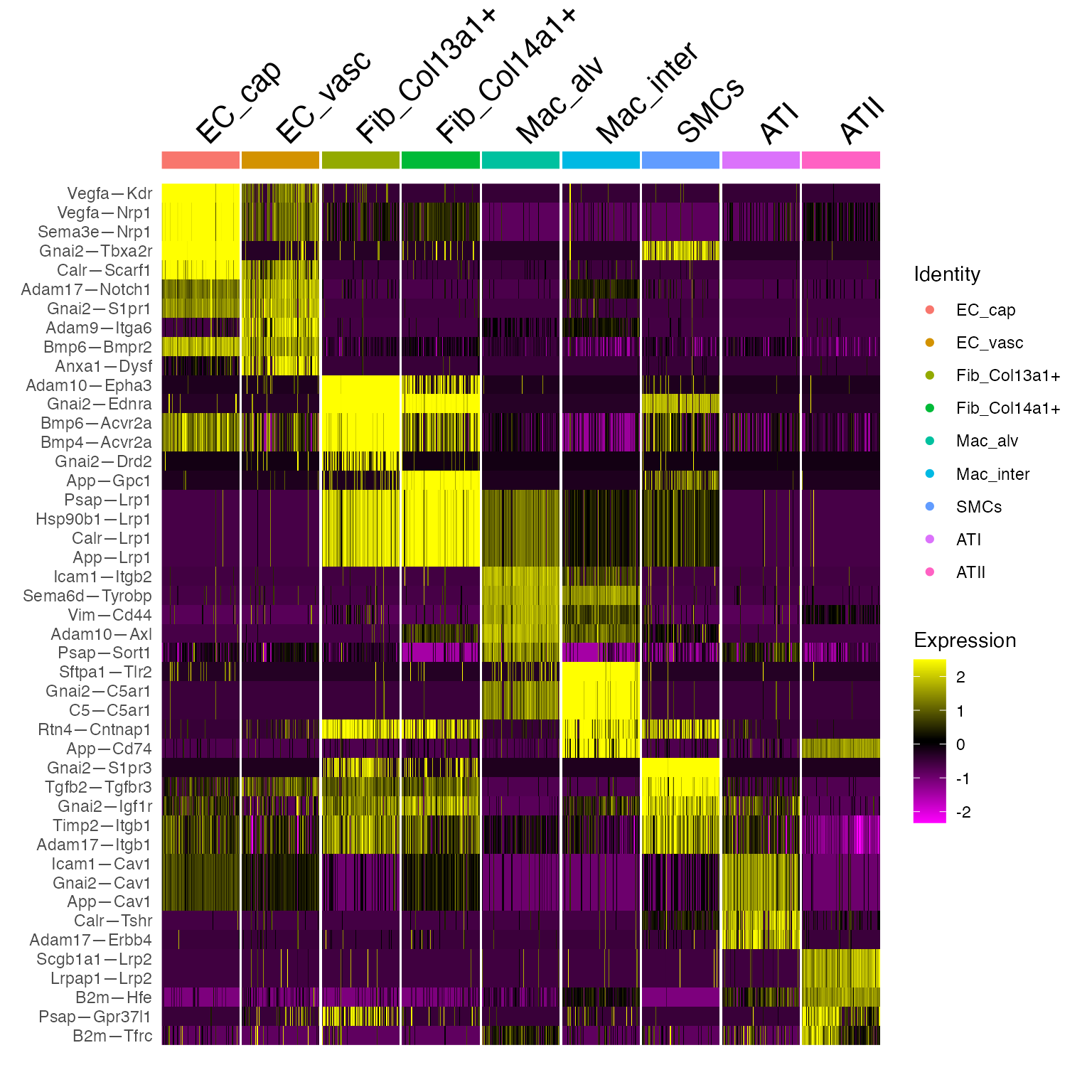
This gives us a sense of the character of each celltype niche. However, it doesn’t allow us to see where the signal is coming from. To ask these kinds of questions, we need to characterize cell-cell relationships, which we do as follows:
lung.cc <- RunNICHES(rat.sub,
                        assay = 'alra',
                        species = 'rat',
                        LR.database = 'fantom5',
                        cell_types = "cell_types",
                        CellToCell = T) #Note the difference in input arguments here
cc.object <- lung.cc$CellToCell #Extract the output of interest
cc.object <- ScaleData(cc.object) #Scale
cc.object <- FindVariableFeatures(cc.object,selection.method="disp") #Identify variable features
cc.object <- RunPCA(cc.object,npcs = 100) #RunPCA
ElbowPlot(cc.object,ndims=100) #Choose PCs to use for embedding
cc.object <- RunUMAP(cc.object,dims = 1:100) #Embed
DimPlot(cc.object,reduction = 'umap',label = F)+ NoAxes()+ ggtitle('Alveolar Cell-Cell Signaling')+
  guides(colour=guide_legend(ncol=2,override.aes = list(size=6))) #Plot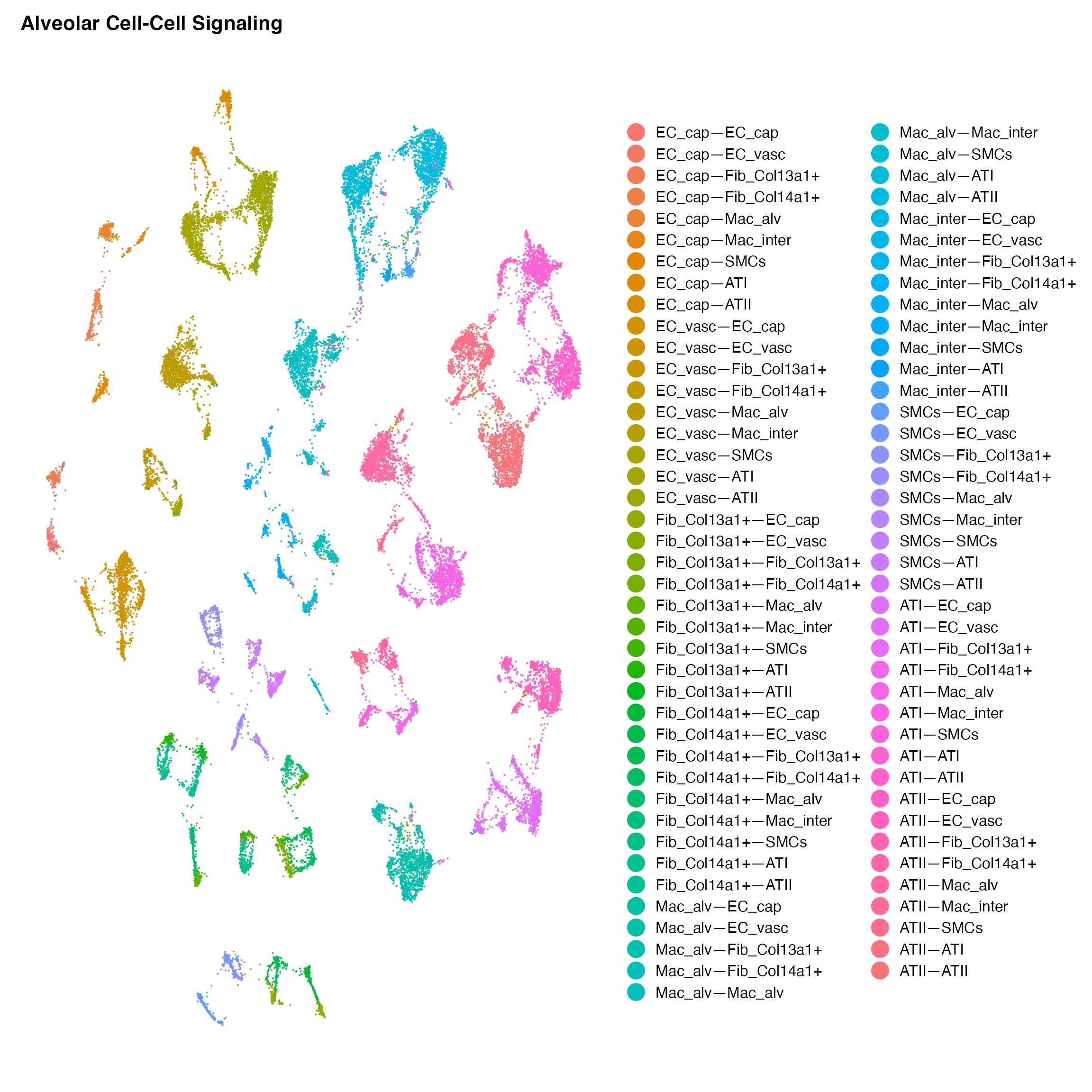
We are now prepared to fully dissect a given cellular niche. Let’s see how different cells influence the EC_cap population within this system:
Idents(cc.object) <- cc.object[['ReceivingType']]
ec.network <- subset(cc.object,idents ='EC_cap')
Idents(ec.network) <- ec.network[['VectorType']]
mark.ec <- FindAllMarkers(ec.network,
                          logfc.threshold = 1,
                          min.pct = 0.5,
                          only.pos = T,
                          test.use = 'roc')
# Pull markers of interest to plot
mark.ec$ratio <- mark.ec$pct.1/mark.ec$pct.2
marker.list.ec <- mark.ec %>% group_by(cluster) %>% top_n(5,avg_log2FC)

#Plot in Heatmap form
DoHeatmap(ec.network,features = marker.list.ec$gene,cells = WhichCells(ec.network,downsample = 100))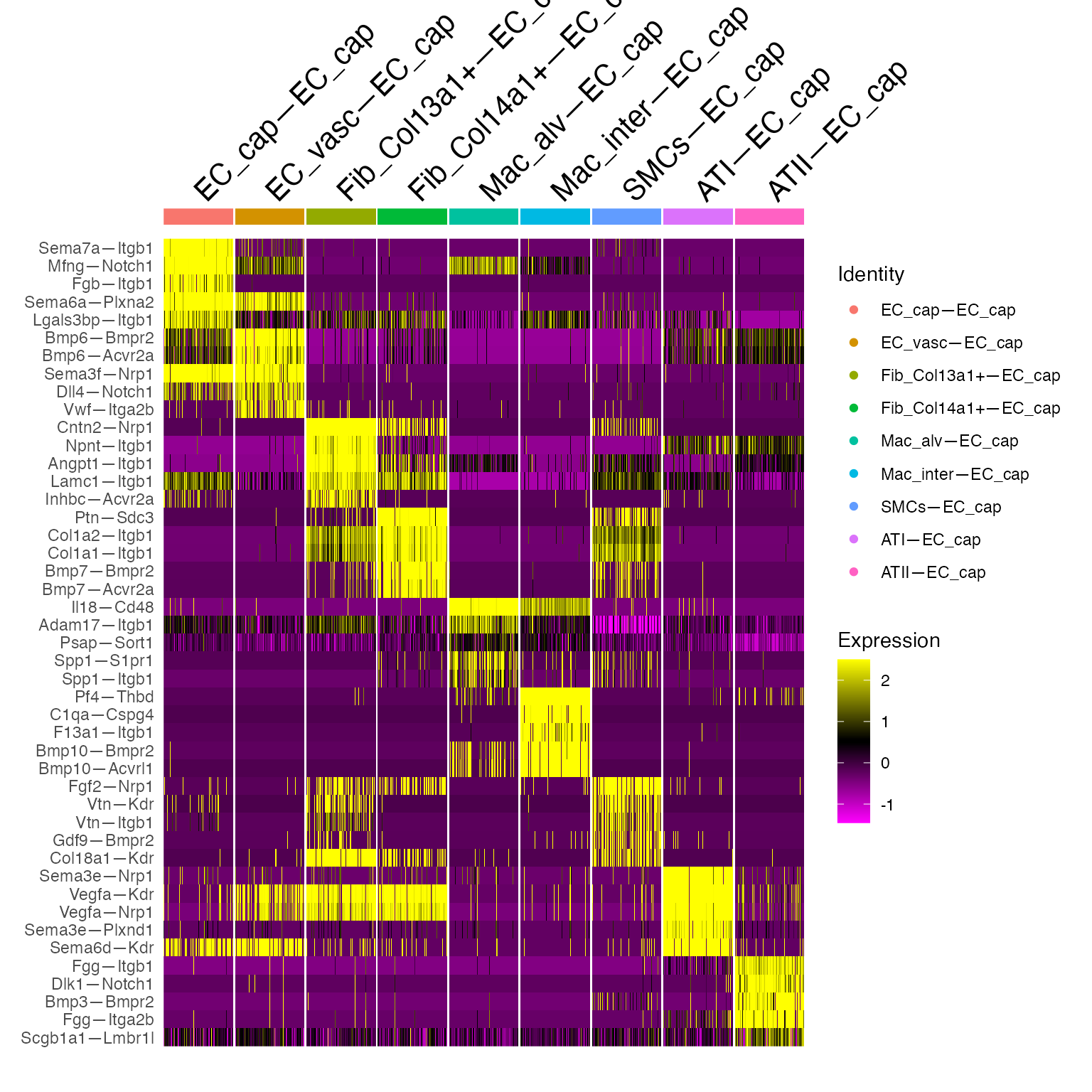
One of the powerful applications of NICHES is the ability to parse intra-cluster heterogeneity very easily, to see if there are subtly-different subcategories of cell-cell relationships present within the data. Here, we further dissect cell-cell signaling coming from alveolar macrophages and landing on the ATI cell population:
# Subclustering of a relationship:
Idents(cc.object) <- cc.object[['VectorType']]
sub <- subset(cc.object,idents = 'Mac_alv—ATI')
sub <- ScaleData(sub)
sub <- FindVariableFeatures(sub,selection.method="disp")
sub <- RunPCA(sub)
ElbowPlot(sub,ndims=50)
PCHeatmap(sub,dims=1:10,balanced = T,cells=100)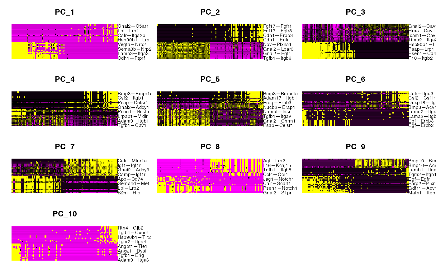
sub <- RunUMAP(sub,dims = 1:10)
sub <- FindNeighbors(sub,dims = 1:10,force.recalc = T)
sub <- FindClusters(sub,resolution = 0.1)
#> Modularity Optimizer version 1.3.0 by Ludo Waltman and Nees Jan van Eck
#>
#> Number of nodes: 1331
#> Number of edges: 40995
#>
#> Running Louvain algorithm...
#> Maximum modularity in 10 random starts: 0.9292
#> Number of communities: 5
#> Elapsed time: 0 seconds
DimPlot(sub)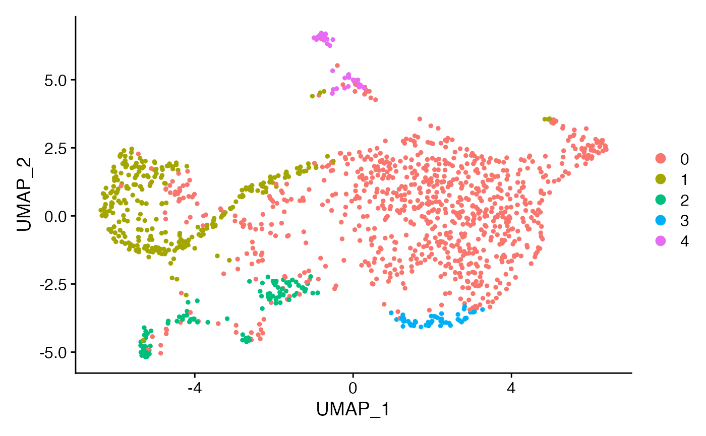
This looks interesting. Let’s explore some marker mechanisms:
mark.sub <- FindAllMarkers(sub,only.pos = T,test.use = 'roc')
marker.sub.list <- mark.sub %>% group_by(cluster) #%>% top_n(20,avg_log2FC)
DoHeatmap(sub,features = marker.sub.list$gene)+
  scale_fill_gradientn(colors = c("grey","white", "blue"))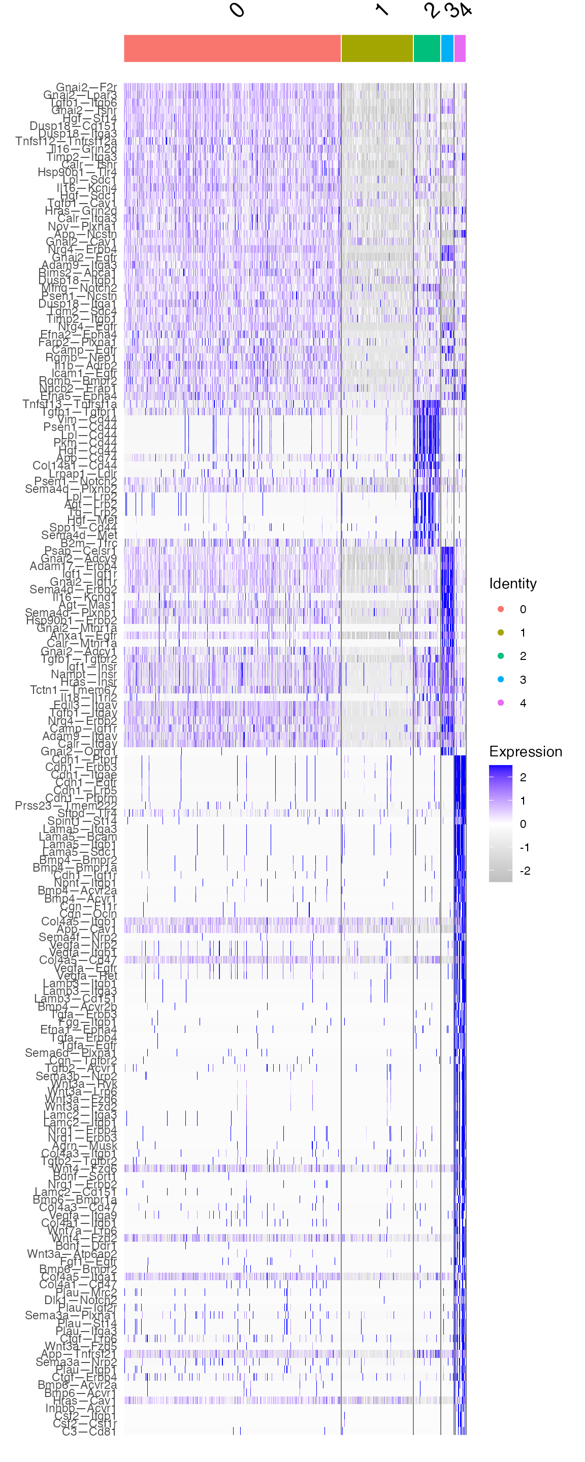
All of these measurements are from the pairing of an alveolar macrophage as a sending cell and an ATI cell as a receiving cell. However, within this single cell-cell relationship, there are subcategories of cell pairings which are possible. Above, it is notable that cluster 1 is quite sparse in mechanism employment. Additionally, cluster 4 is employing a number of signaling mechanisms which are largely not used by the other subcategories of macrophage-ATI pairings.