Here, we show how NICHES can be used to compare cellular microenvironment change between different time points in spatial transcriptomic data.

First, let’s load dependencies.

Load Required Packages

library(Seurat)
library(NICHES)
library(ggplot2)
library(dplyr)
library(cowplot)

The data we will be using is the E10 and E11 mouse embryonic eye region dbit-seq data demonstrated in Liu, Yang, et al. “High-spatial-resolution multi-omics sequencing via deterministic barcoding in tissue.” Cell 183.6 (2020): 1665-1681. The data are processed using the original pipeline and then imputed by ALRA.

Load Data

load("spatial_e10_processed_alra.Robj")
load("spatial_e11_processed_alra.Robj")

Let’s visualize the data on top of the spatial grids.

Visualize Data

ggplot(data = E10@meta.data,aes(x=x,y=y,color=cell_label_dom))+
  geom_point(size=2)+
  scale_color_brewer(palette="Paired")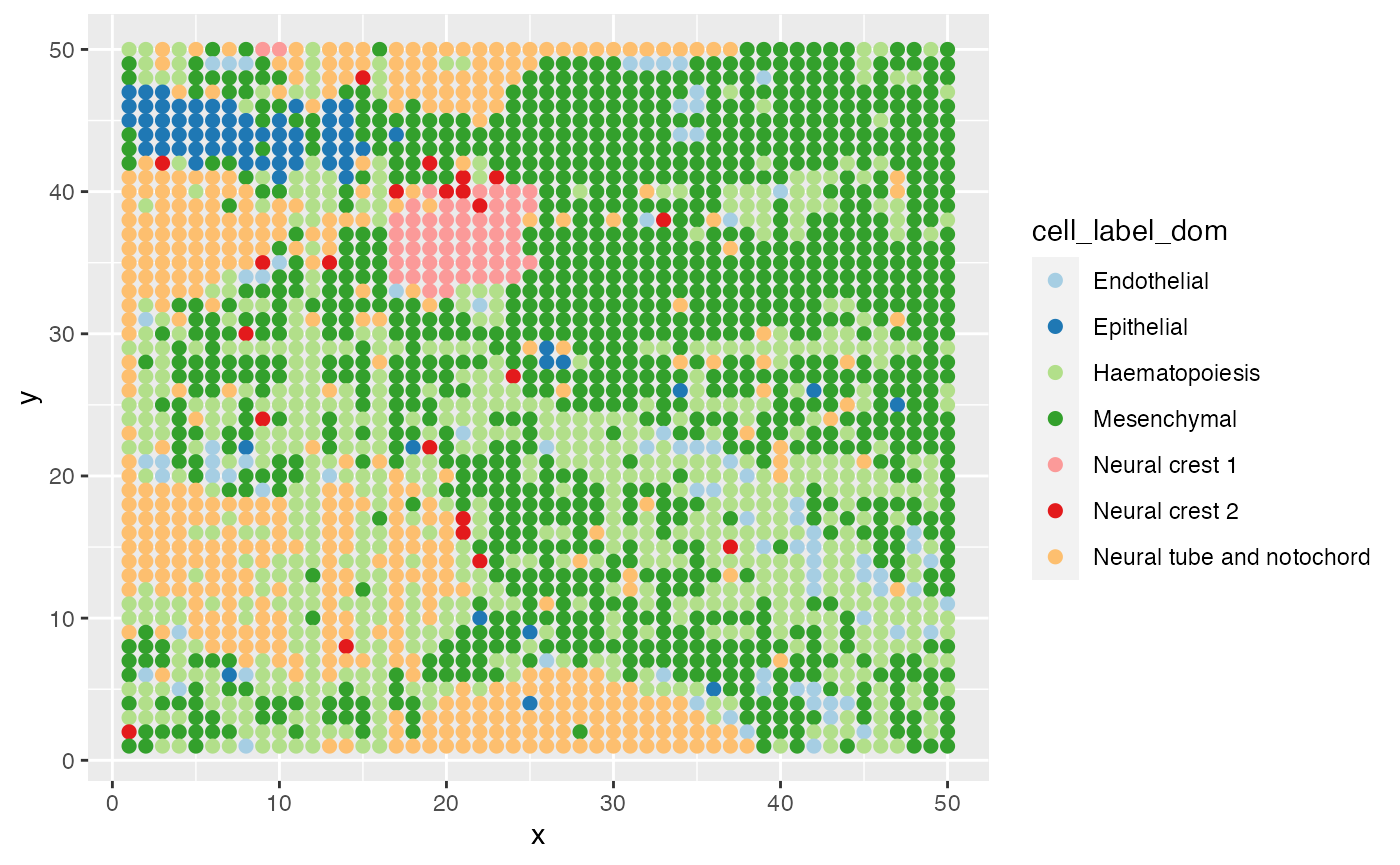

ggplot(data = E11@meta.data,aes(x=x,y=y,color=cell_label_dom))+
  geom_point(size=2)+
  scale_color_brewer(palette="Paired")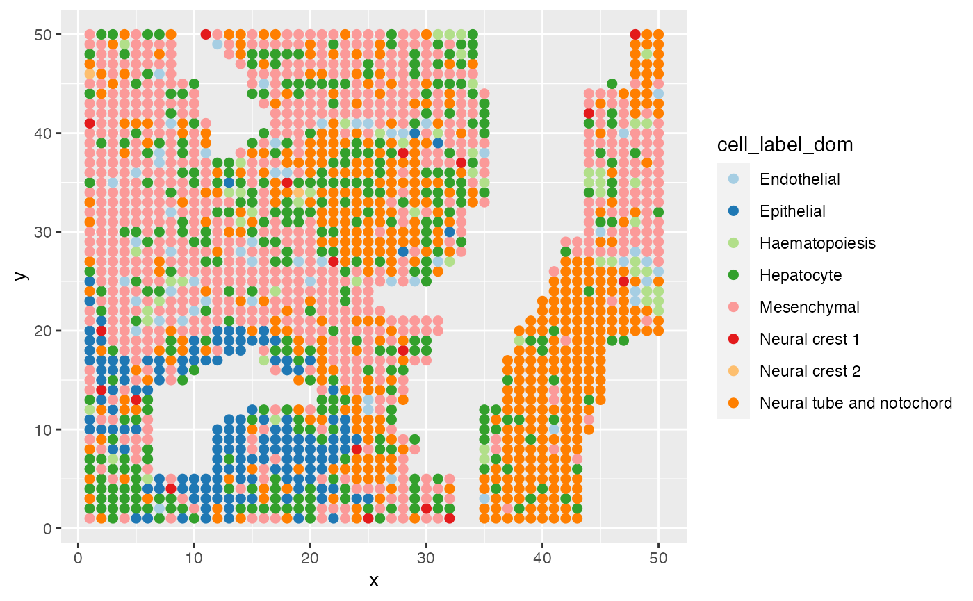

NICHES can be run on imputed or non-imputed data. Here, we will run NICHES on each sample using imputed data.

Run NICHES on each sample

# Put objects in a named list together
data.list <- list(E10,E11)
names(data.list) <- c('E10','E11')
# Run NICHES on each item in list and store the output
niches.list <- list()
for (i in 1:length(data.list)){

data.list[[i]]@meta.data$cell_types <- Idents(data.list[[i]])  
  
niches.list[[i]] <- RunNICHES(data.list[[i]],
                 assay = 'alra', # Note: using alra imputed data here instead of SCT
                 species = 'mouse',
                 LR.database = 'fantom5',
                 cell_types = "cell_types",
                 CellToCellSpatial = T, # We are interested in local relationships
                 NeighborhoodToCell = T, # We are interested in local niches
                 CellToCell = F, # We do not want crosses which don't take into account spatial information
                 position.x = "x",
                 position.y= "y",
                  )
}
names(niches.list) <- names(data.list)

NICHES outputs a list of objects. Each object contains a certain style of cell-system signaling atlas. Above, we computed both spatial cell to cell interactions and individual cellular microenvironment. We next isolate this output and focus on the spatial microenvironemnt of each cell. Then we can visualize the data on UMAP after the processing steps.

Investigate local microenvironment

# Extract output of interest
menv <- list()
for (i in 1:length(niches.list)){
  menv[[i]] <- niches.list[[i]][["NeighborhoodToCell"]] # Extract microenvironment information
  menv[[i]]$Condition <- names(niches.list)[i]
}
# Merge together
menv <- merge(menv[[1]],menv[2])
table(menv$Condition,menv$ReceivingType)
#>      
#>       Endothelial Epithelial Haematopoiesis Hepatocyte Mesenchymal
#>   E10          85         71            658          0        1146
#>   E11          57        152             58        346         701
#>      
#>       Neural crest 1 Neural crest 2 Neural tube and notochord
#>   E10             56             22                       462
#>   E11             18              2                       506

# Scale
menv <- ScaleData(menv)
# Find variable features
menv <- FindVariableFeatures(menv,selection.method = "disp")
# Run PCA
menv <- RunPCA(menv,npcs = 100) # Run PCA
ElbowPlot(menv,ndims = 100)

PCHeatmap(menv,dims = 40:48,cells=100,balanced=T)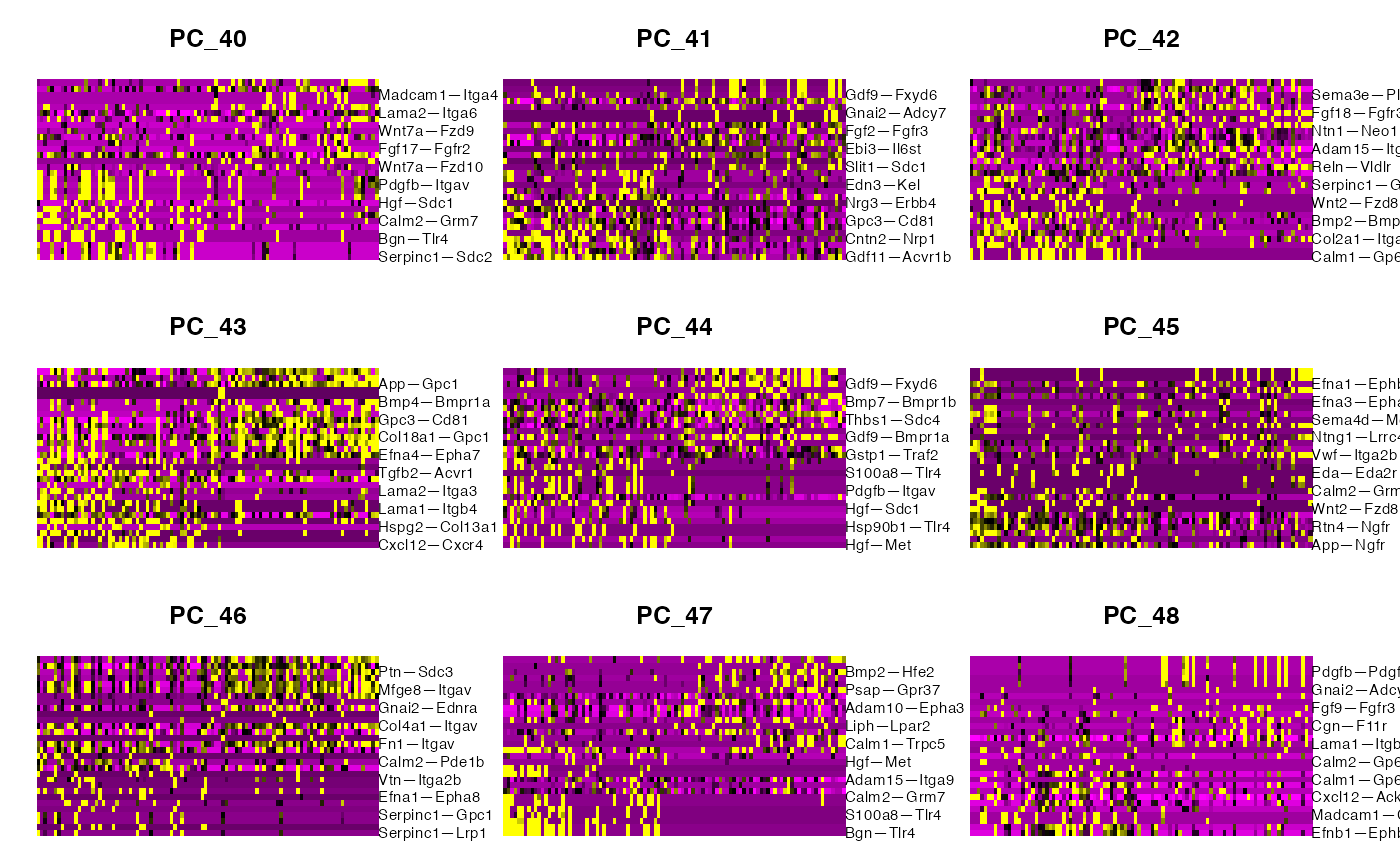

menv <- RunUMAP(menv,dims = 1:50)
p1 <- DimPlot(menv)+ggtitle('ReceivingType')
p2 <- DimPlot(menv,group.by = 'Condition')
plot_grid(p1,p2,ncol=1)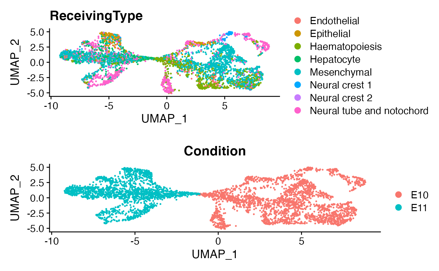

Here as a demonstration, we focus on a specific cell population, namely “Neual tube and notochord”.

Isolate a ReceivingType of interest

ROI <- "Neural tube and notochord"
subs <- subset(menv,idents = ROI)
# Scale
subs <- ScaleData(subs)
# Find variable features
subs <- FindVariableFeatures(subs,selection.method = "disp")
# Run PCA
subs <- RunPCA(subs,npcs = 50) # Run PCA
ElbowPlot(subs,ndims = 50)

PCHeatmap(subs,dims = 30:38,cells=100,balanced=T)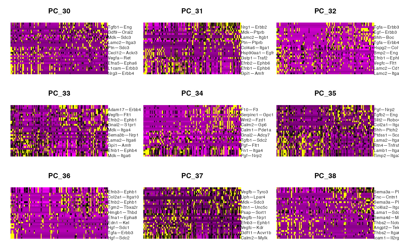

subs <- RunUMAP(subs,dims = 1:40)
p1 <- DimPlot(subs)+ggtitle('ReceivingType')
p2 <- DimPlot(subs,group.by = 'Condition')
plot_grid(p1,p2,ncol=1)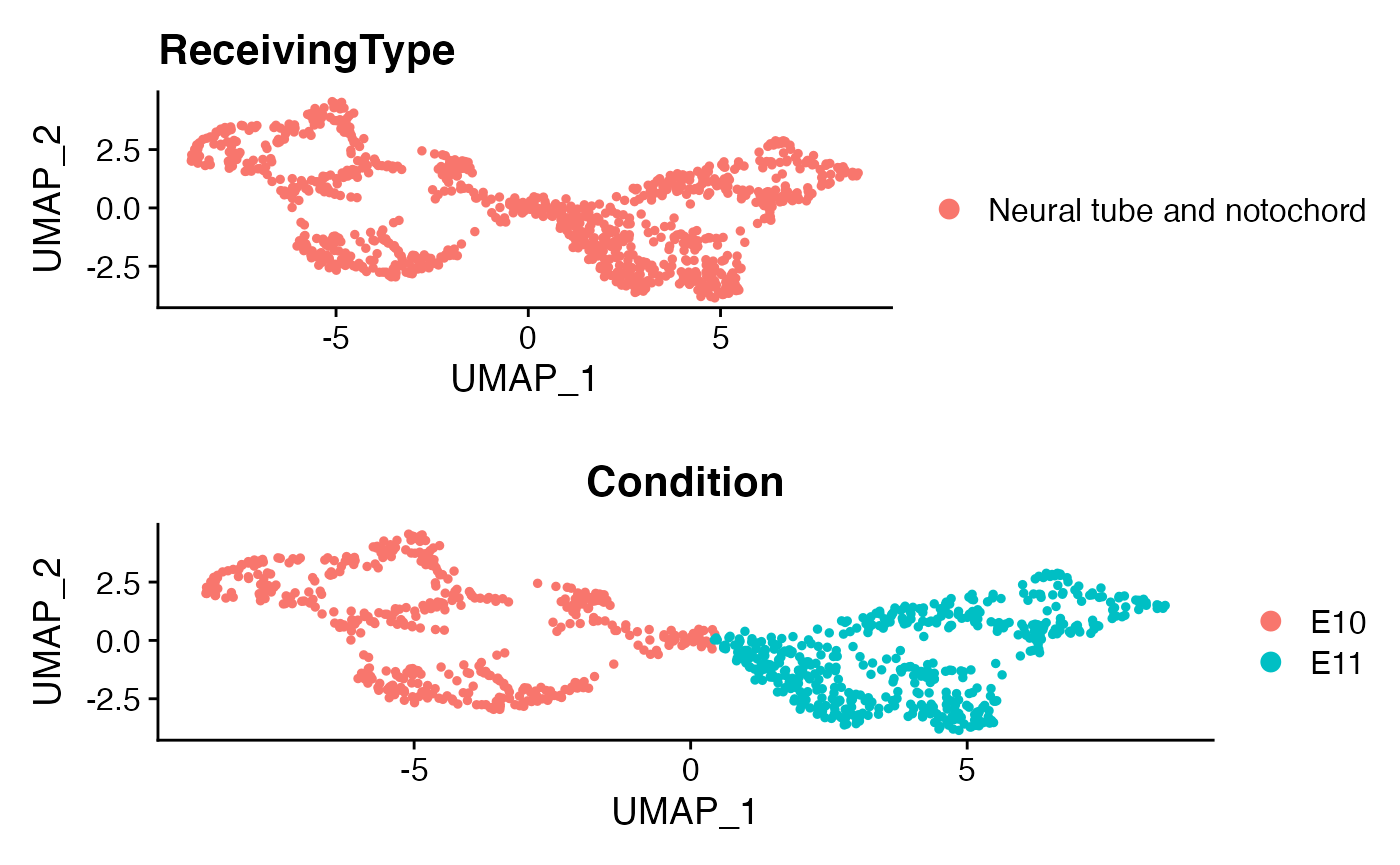

With the NICHES framework, we can very easily perform differential ligand-receptor interaction analysis between the time points. We can also visualize the top markers in different visualization plots.

Differential Analysis of Neural Tube Microenvironment

Idents(subs) <- subs[['Condition']]
marker.subs <- FindAllMarkers(subs,min.pct = 0.25,only.pos = T,test.use = "roc")
# Remove markers mapped in only one dataset (infinite differential)
marker.subs$ratio <- marker.subs$pct.1/marker.subs$pct.2
marker.subs <- marker.subs[marker.subs$ratio < Inf,]
# Select top markers
GOI_niche.subs <- marker.subs %>% group_by(cluster) %>% top_n(20,myAUC)
# Make a heatmap
DoHeatmap(subs,
          group.by="ident",
          features=GOI_niche.subs$gene)+
  ggtitle("Top DE Mechanisms, Neural Tube Microenvironment, E10 vs E11")+
  theme(plot.title = element_text(vjust = 5))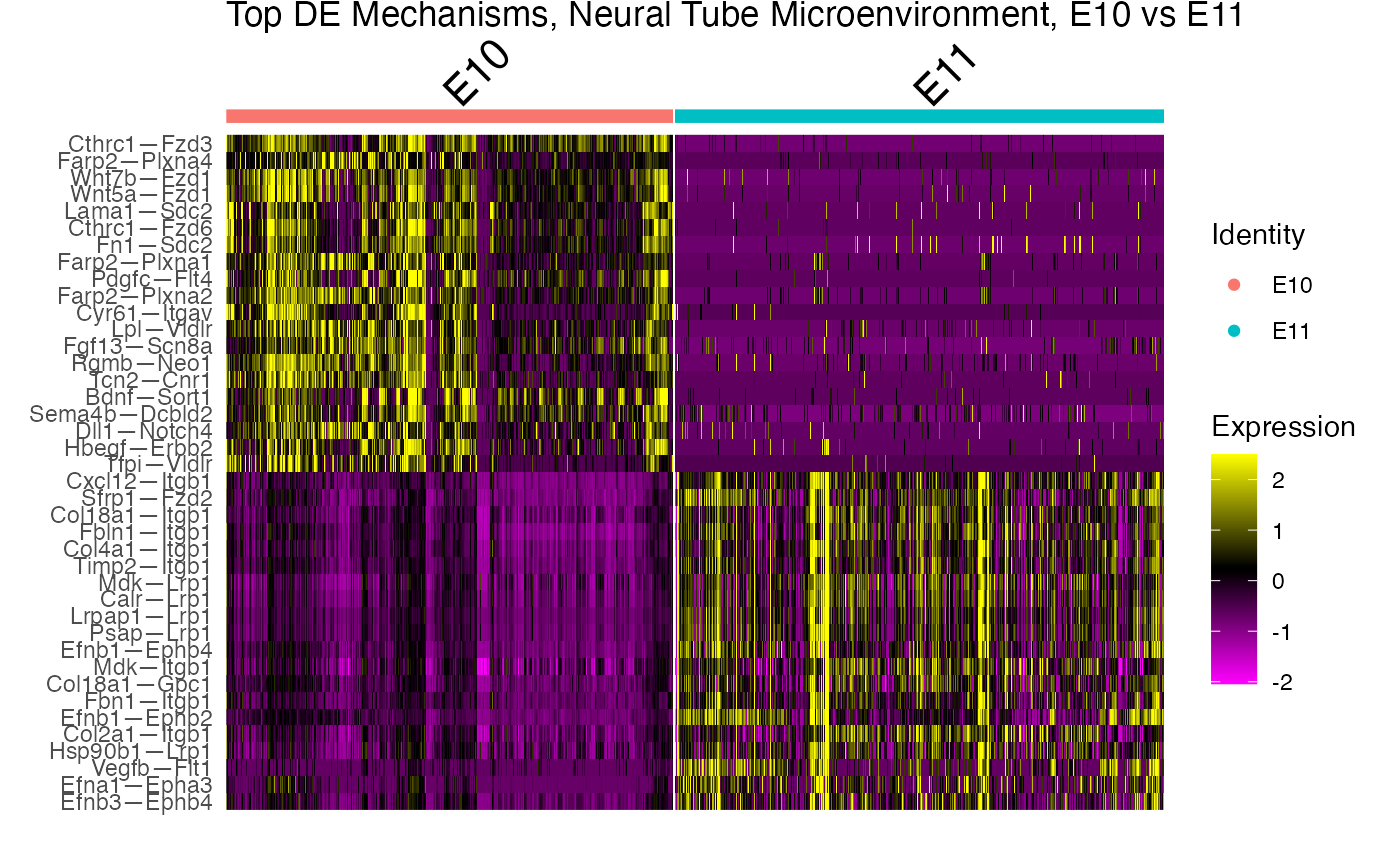

FeaturePlot(subs,'Dll1—Notch4')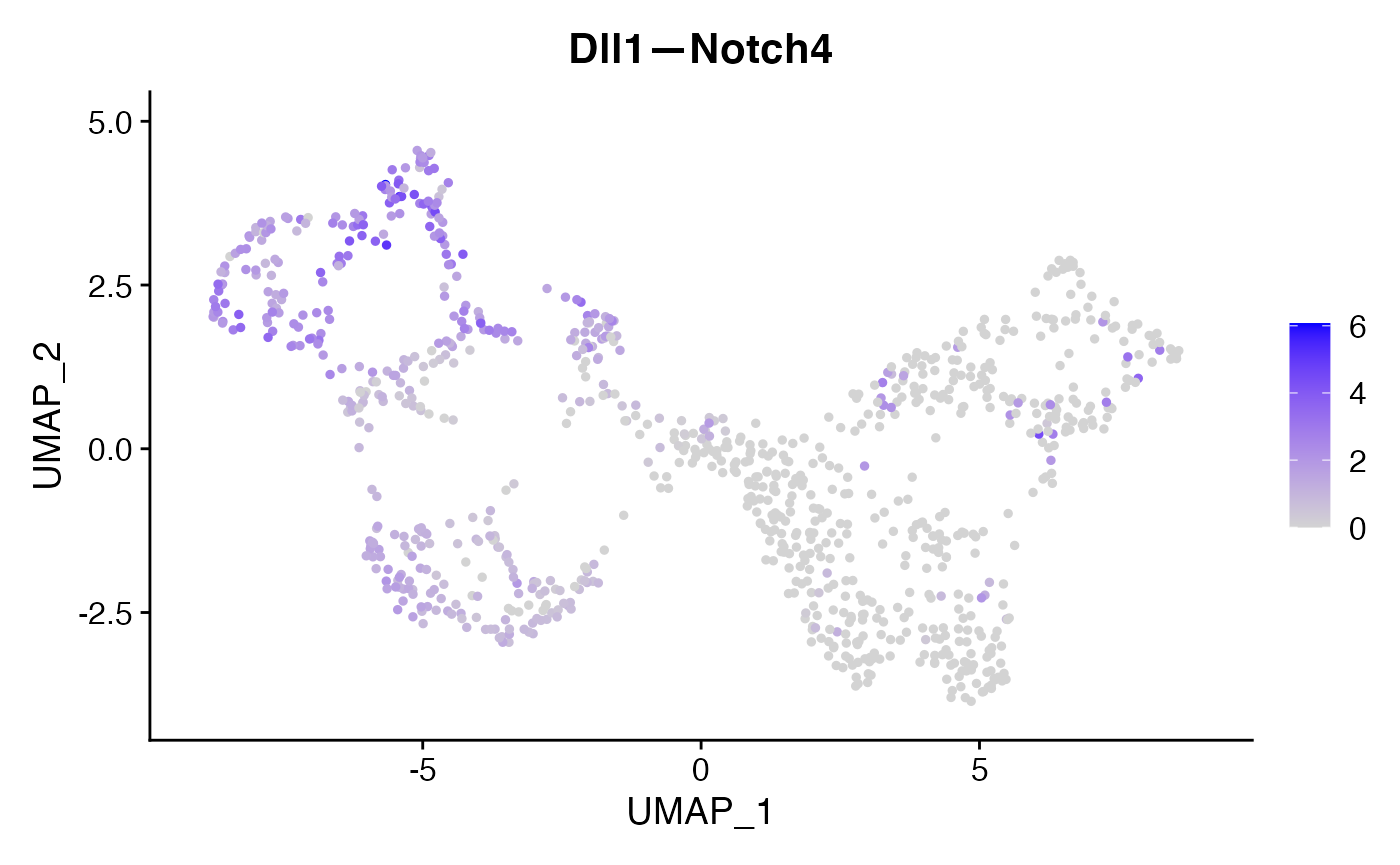

For this identified Dll1—Notch4 interaction, we can incorporate the NICHES output back to the original data as a new assay and visualize their interaction levels along with the corresponding gene expression levels.

Add Niches microenvironment output as an assay in the original data

# Extract tabular data and annotate with receiving cell barcodes
niches.data <- list()
for (i in 1:length(niches.list)){
  niches.data[[i]] <- GetAssayData(object =  niches.list[[i]][['NeighborhoodToCell']], slot = 'data')
  colnames(niches.data[[i]]) <- niches.list[[i]][['NeighborhoodToCell']]@meta.data$ReceivingCell
}
# Add as a new assay
for (i in 1:length(data.list)){
  data.list[[i]][["NeighborhoodToCell"]] <- CreateAssayObject(data = niches.data[[i]])
  DefaultAssay(data.list[[i]]) <- "NeighborhoodToCell"
  data.list[[i]] <- ScaleData(data.list[[i]])
}
# Merge the timepoints together to visualizejointly
merge <- merge(data.list[[1]],data.list[2])

# View change in microenvironment for all celltypes and for specific celltype of interest
VlnPlot(merge,'Dll1—Notch4',assay = "NeighborhoodToCell",split.by = 'orig.ident')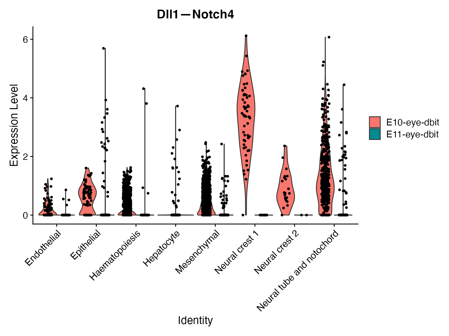

VlnPlot(merge,idents = ROI,'Dll1—Notch4',assay = "NeighborhoodToCell",split.by = 'orig.ident')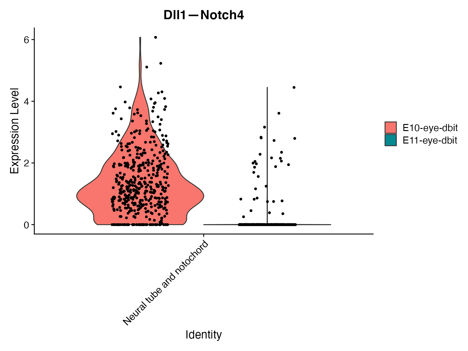


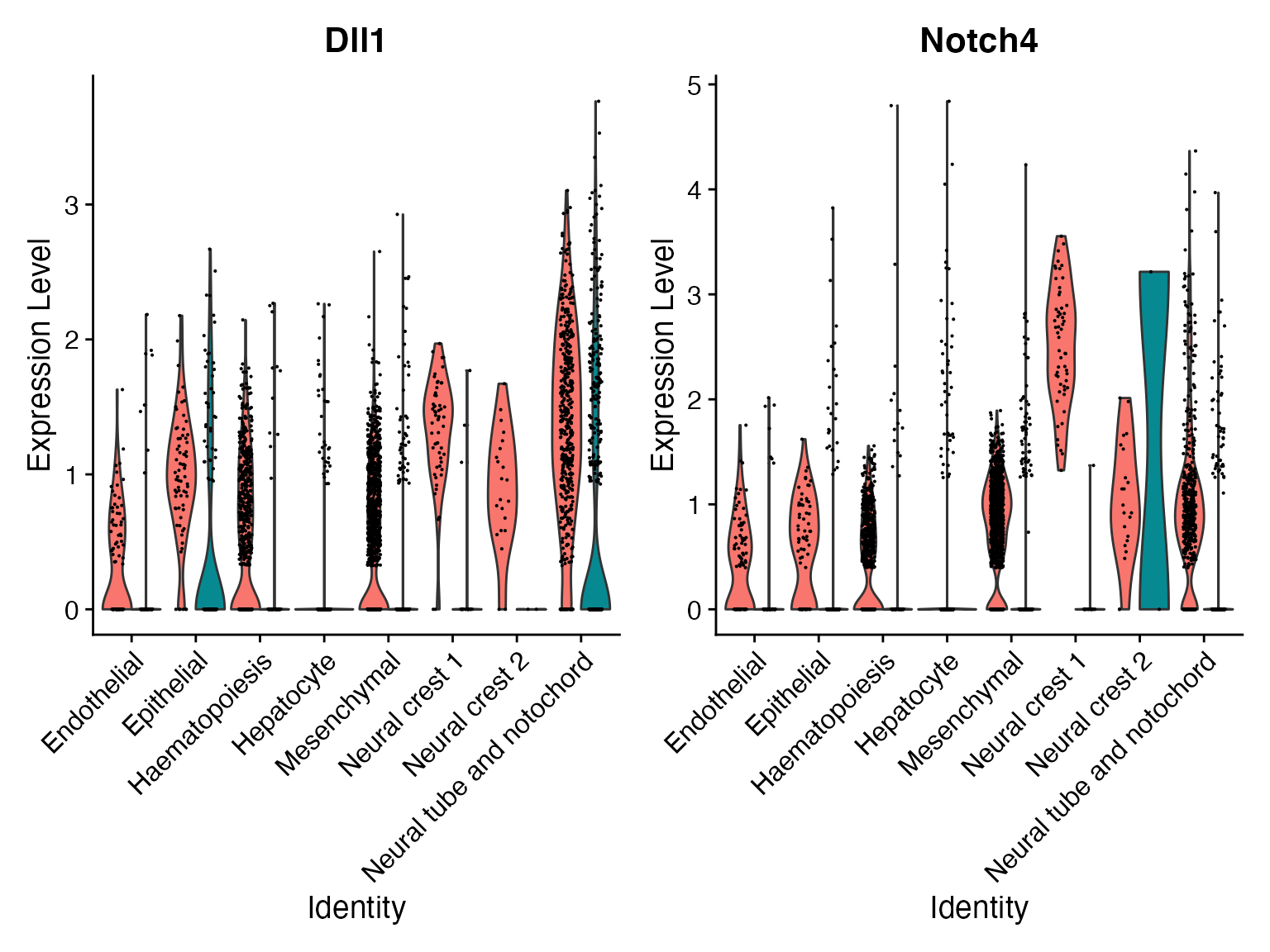
# View change in ligand and receptor expression for all celltypes to better understand origin of the above signal differential
VlnPlot(merge,c('Dll1','Notch4'),assay = 'alra',split.by = 'orig.ident')

Spatio-Temporal NICHES

Junchen Yang & Micha Sam Brickman Raredon

2022-07-20